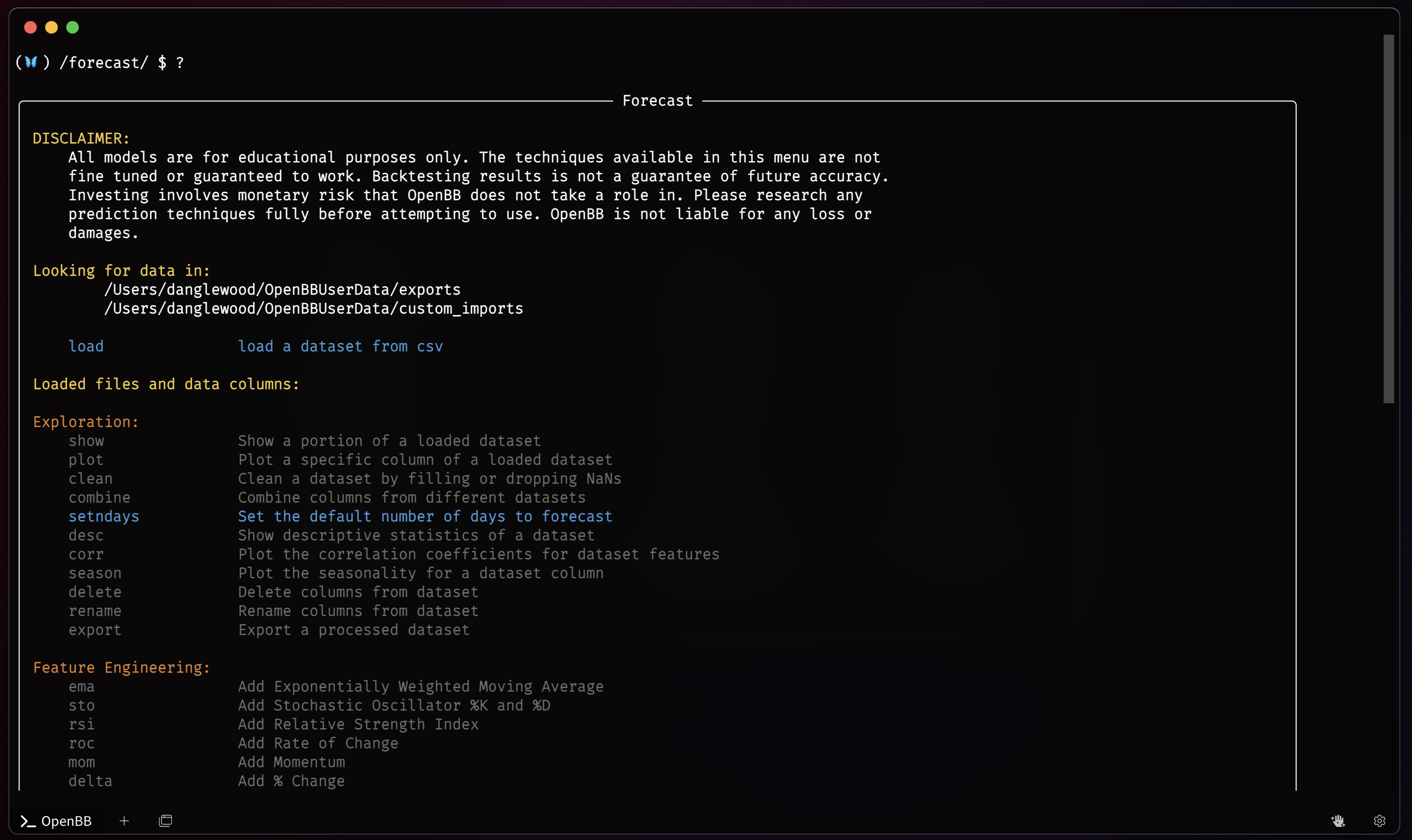
Forecast

The Forecast menu is a machine learning toolkit that provides practitioners with high-level, state-of-the-art, components. Classical or deep learning models can be combined with low-level components and fine tuned to build new approaches and custom tuned models. Bring in multiple datasets and train machine learning models with unlimited external factors to see how underlying data may change future forecasting predictions and accuracy.

Usage

The Forecast menu is entered from the Main menu, forecast, or with the absolute path:

 /forecast

There are also methods for entering the menu with a loaded ticker symbol from either of the /crypto menu and /stocks menu

The menu is divided into sections for:

• Loading Data
• Data Exploration
• Feature Engineering
• Time Series Forecasting
• Anomaly Detection
• Miscellaneous AI Tools

and the functions within these groups are described in the following sections.

Loading Data

With the Load Command

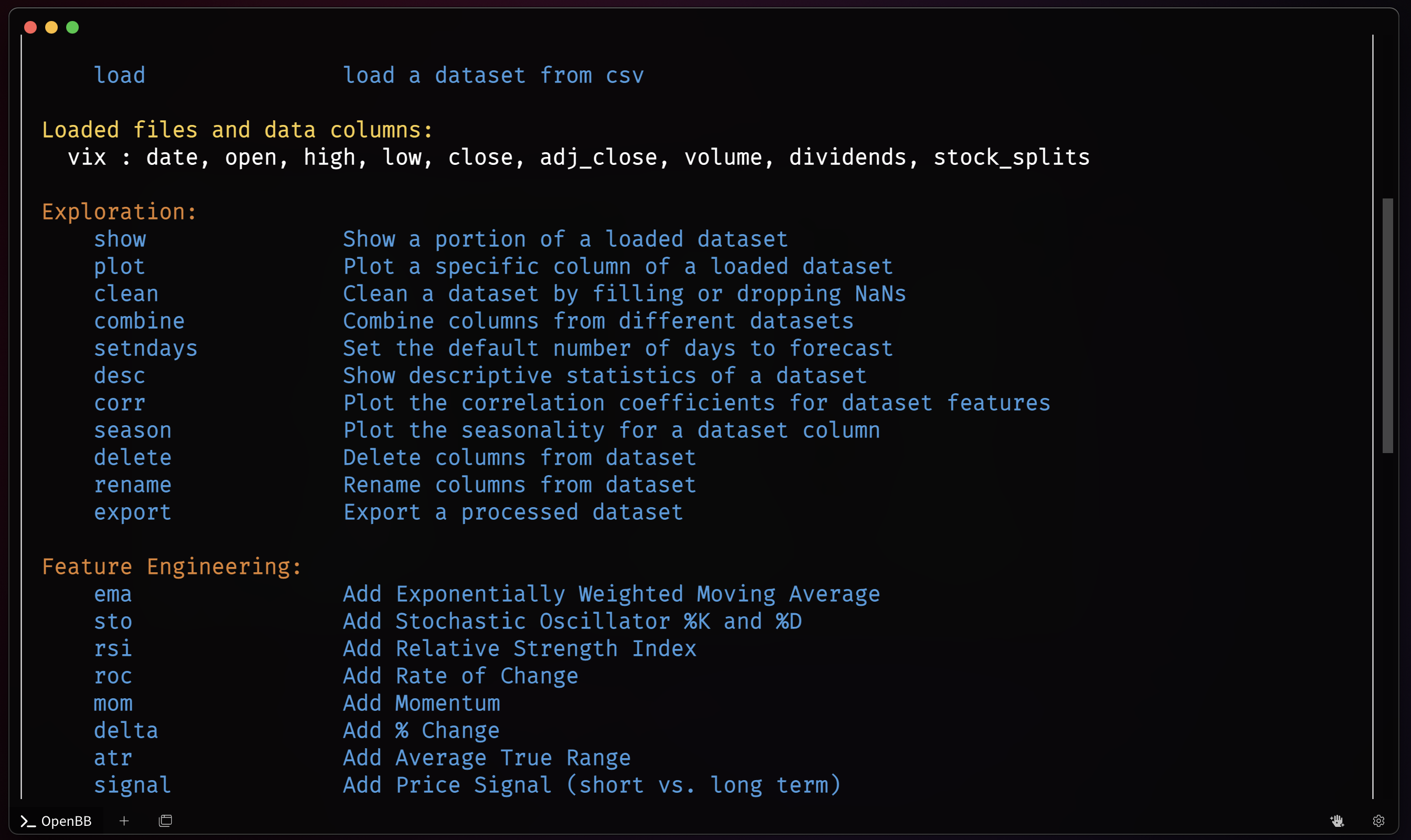
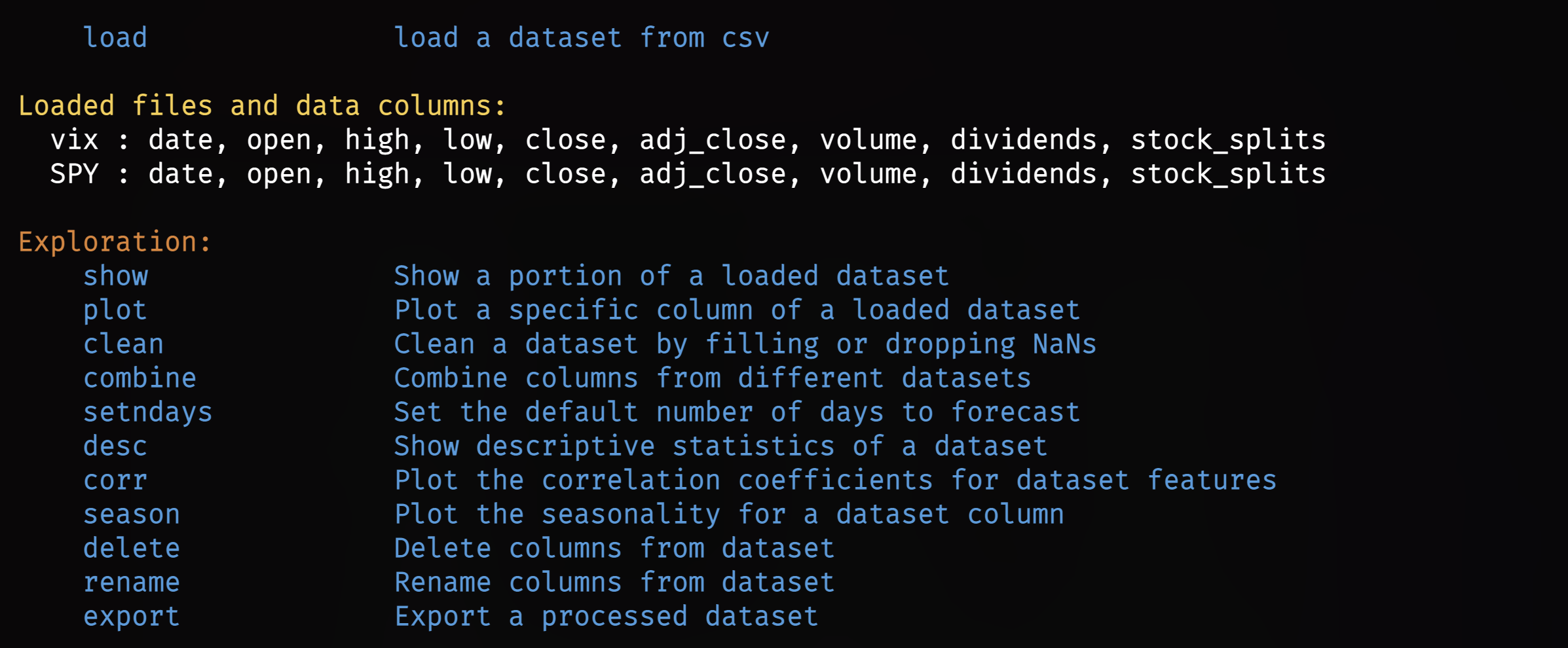
If the Forecast menu has not been entered directly through the /crypto or /stocks menus, a dataset must be loaded before commencing any work. Use the load command to open one from a CSV file placed in the OpenBBUserData folder. The paths where the auto completion engine is looking for files is printed on the screen directly above the load command, Looking for data in:

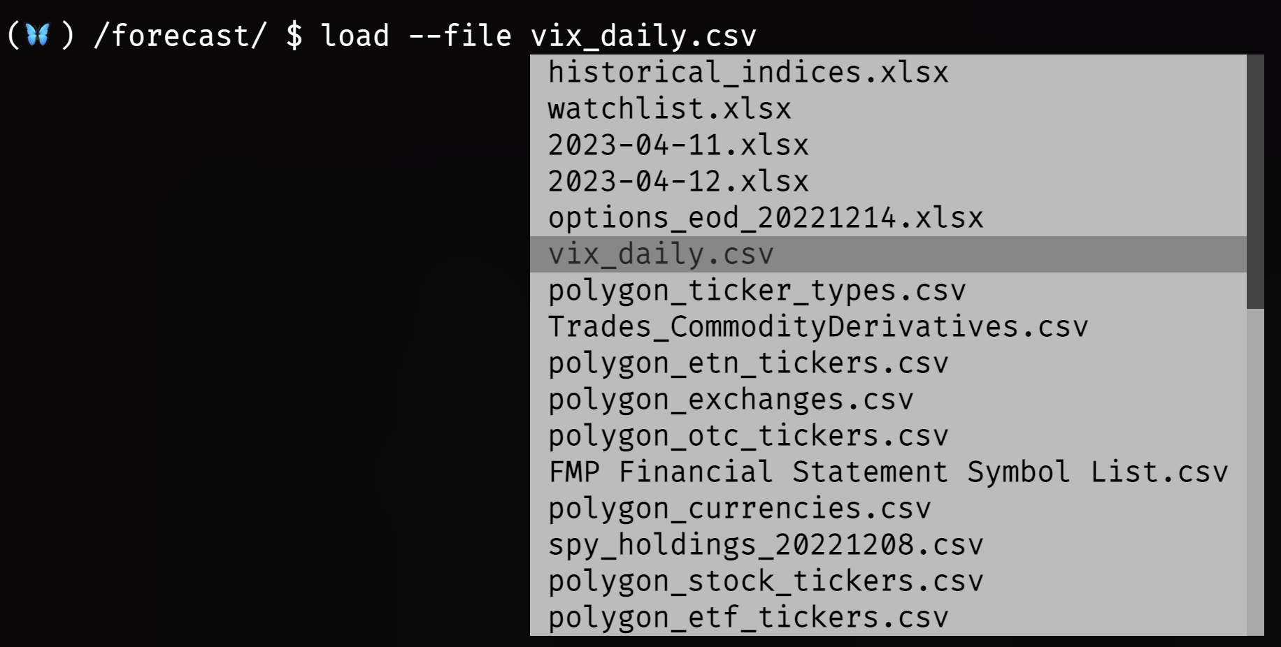
Use the following syntax to load a file and name a dataset, substituting vix_daily with the name of the file.

load --file vix_daily.csv --alias vix

To refresh the screen, enter: ?

The dataset will be listed under the load command and display the column names within it.

Repeat the process until all desired datasets have been loaded.

Via the Stocks/Crypto Menus

Use the load command, according to the nuances of each menu. For example's sake, and to match the starting date of the previously loaded file, it will look like:

/stocks/load SPY --start 1997-01-01/forecast

Combine these two methods an unlimited number of times for building a more complex model and forecast.

With some data loaded, the first series of tools are for inspecting, managing, and exporting the sets.

Exploration

The exploration functions are listed in the table below, along with a short description.

Function	Description
clean	Clean a dataset by filling or dropping NaNs.
combine	Combine columns from different datasets.
corr	Plot the correlation coefficients for dataset features.
delete	Delete columns from dataset.
desc	Show descriptive statistics of a dataset.
export	Export a processed dataset.
plot	Plot a specific columns of a loaded dataset.
rename	Rename columns from dataset.
season	Plot the seasonality for a dataset column.
setndays	Set the default number of days to forecast.
show	Show a portion of a loaded dataset.

Combine

When running a model, all targeted columns must be within the same dataset. Use the combine command to accomplish this by merging one column with another dataset.

combine --dataset SPY -c vix.high
combine --dataset SPY -c vix.low

The SPY time series now has two additional columns from the VIX dataframe, high and low.

Delete

It may be desirable to remove entire columns from the target dataset. The syntax below removes the three columns from the SPY data loaded through the stocks menu.

delete --delete SPY.adj_close
delete --delete SPY.stock_splits
delete --delete SPY.dividends

Show

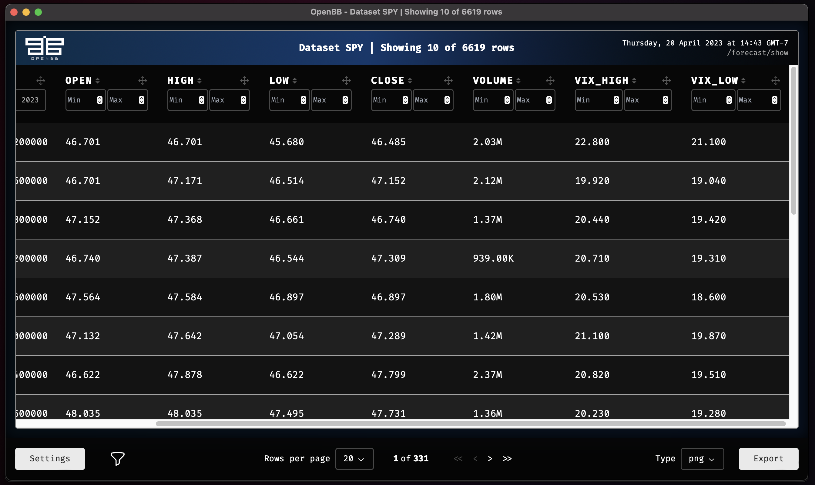
After performing operations, examine the results using the show command.

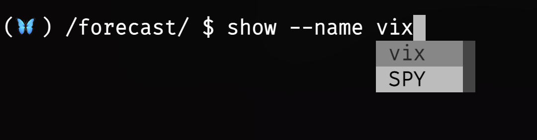
show --name SPY

Export

To save all of the combined changes within a dataset, export it to a new file.

export -d SPY --type csv

This creates a new file in the OpenBBUserData folder.

Feature Engineering

The Feature Engineering section provides methods for making fast calculations with a dataset. Each one is listed below with a short description.

Function	Description
atr	Add Average True Range
delta	Add % Change
ema	Add Exponentially Weighted Moving Average
mom	Add Momentum
roc	Add Rate of Change
rsi	Add Relative Strength Index
sto	Add Stochastic Oscillator %K and %D
signal	Add Price Signal (short vs. long term)

Each function will have slight variations to the command syntax, but will generally operate similarly. Print the help dialogue as a reminder.

usage: rsi [-d {vix,SPY}] [-c TARGET_COLUMN] [--period PERIOD] [-h]

Add rsi to dataset based on specific column.

options:
  -d {vix,SPY}, --dataset {vix,SPY}
                        The name of the dataset you want to select (default: None)
  -c TARGET_COLUMN, --target-column TARGET_COLUMN
                        The name of the specific column you want to use (default: close)
  --period PERIOD       The period to use (default: 10)
  -h, --help            show this help message (default: False)


For more information and examples, use 'about rsi' to access the related guide.

usage: atr [--close-col CLOSE_COL] [--high-col HIGH_COL] [--low-col LOW_COL] [-d {vix,SPY}]
           [-c TARGET_COLUMN] [-h]

Add Average True Range to dataset of specific stock ticker.

options:
  --close-col CLOSE_COL
                        Close column name to use for Average True Range. (default: close)
  --high-col HIGH_COL   High column name to use for Average True Range. (default: high)
  --low-col LOW_COL     Low column name to use for Average True Range. (default: low)
  -d {vix,SPY}, --dataset {vix,SPY}
                        The name of the dataset you want to select (default: None)
  -c TARGET_COLUMN, --target-column TARGET_COLUMN
                        The name of the specific column you want to use (default: close)
  -h, --help            show this help message (default: False)

For more information and examples, use 'about atr' to access the related guide.

To use these commands with the default settings, apply the syntax below.

atr -d SPY
rsi -d SPY

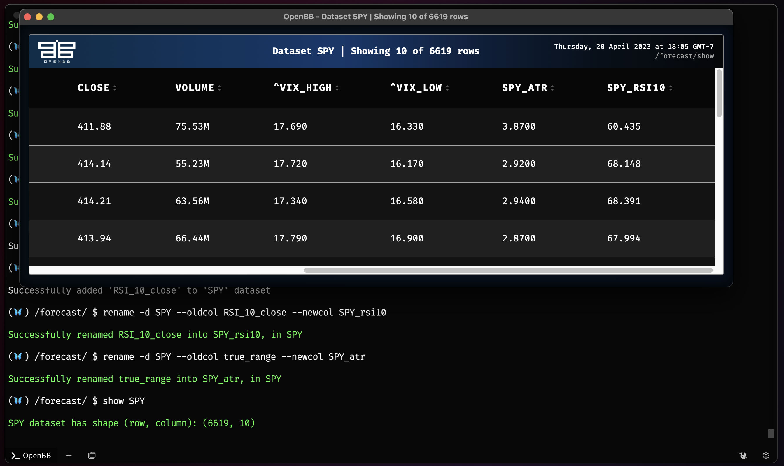
There are now two new columns in the SPY dataset, true_range, RSI_10_close. To keep the dataset organized, it may be worth renaming these columns.

rename -d SPY --oldcol RSI_10_close --newcol spy_rsi10
rename -d SPY --oldcol true_range --newcol spy_atr

Time Series Forecasting

This group of features applies models to a target dataset and its columns. There are a wide selection to choose from. Please note that this guide is meant explain how to use the functions and does not attempt to explain the models themselves. This menu is an implementation of the Unit8 Darts Time Series for Python library.

Function	Description	Accepts Past Covariates?
autoselect	Select best statistical model from AutoARIMA, AutoETS, AutoCES, MSTL, etc.	No
autoarima	Automatic ARIMA Model	No
autoces	Automatic Complex Exponential Smoothing Model	No
autoets	Automatic ETS (Error, Trend, Seasonality) Model	No
mstl	Multiple Seasonalities and Trend using Loess (MSTL) Model	No
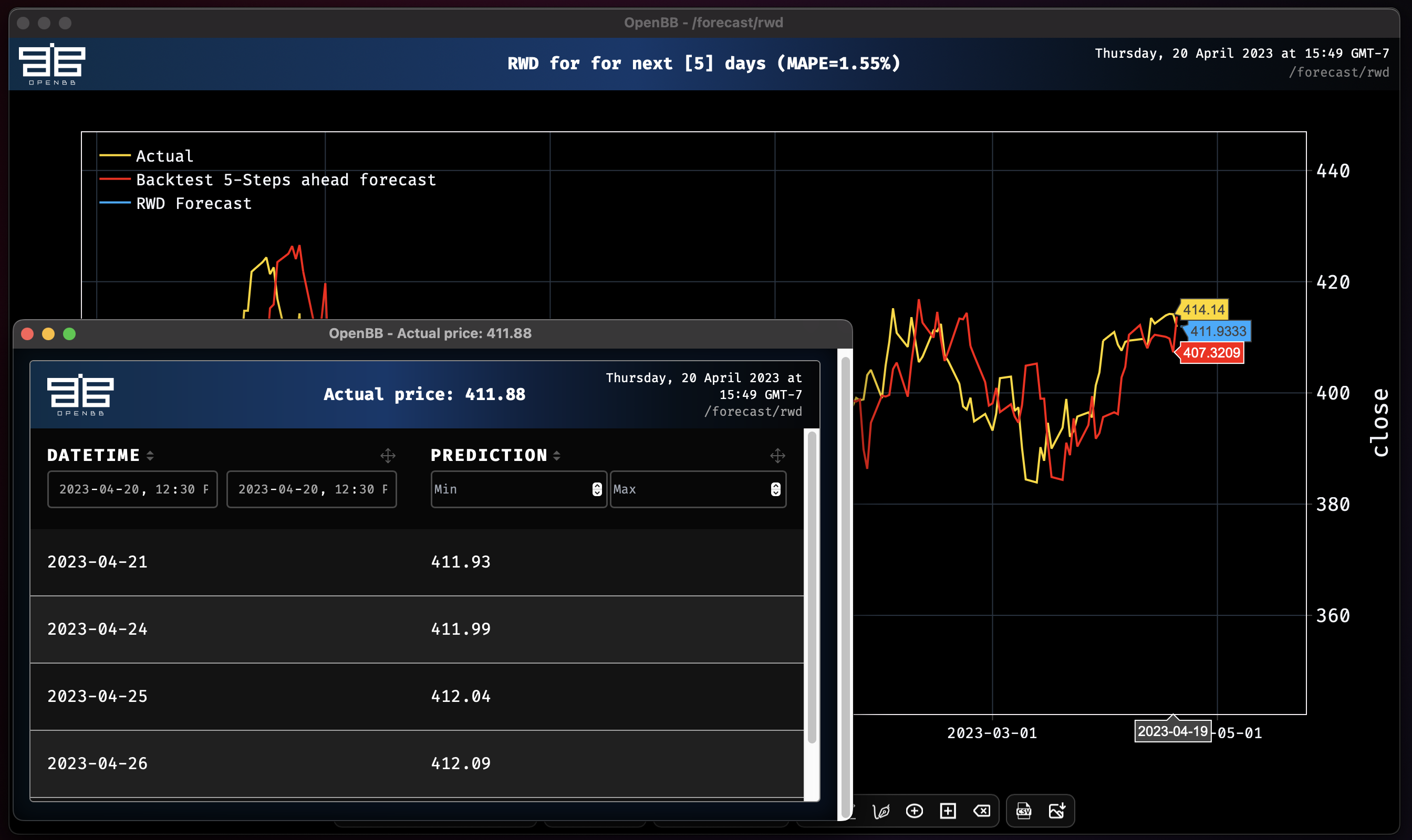
rwd	Random Walk with Drift Model	No
seasonalnaive	Seasonal Naive Model	No
expo	Probabilistic Exponential Smoothing	No
theta	Theta Method	No
linregr	Probabilistic Linear Regression	Yes
regr	Regression	Yes
brnn	Block Recurrent Neural Network (RNN, LSTM, GRU)	Yes
nbeats	Neural Bayesian Estimation	Yes
nhits	Neural Hierarchical Interpolation	Yes
tcn	Temporal Convolutional Neural Network	Yes
trans	Transformer Network	Yes
tft	Temporal Fusion Transformer Network	Yes

Within this list of models, there are two distinct categories:

• Without past covariates.
• With past covariates.

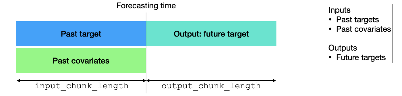
The models featuring past covariates will accept an unlimited number of columns, or all columns can be chosen. The latter being more appropriate for when a dataset contains only columns which are deemed fit for the purpose. To use any model in its default state, all that is required is the command name and the target dataset's name. The default target column will always be close so, a column must be defined to run a model if the target dataset does not contain a column with this name. With the target column as close, the basic default syntax will look like:

rwd -d SPY

Each model should be reviewed carefully to understand what the adjustable parameters are, and how they should be defined.

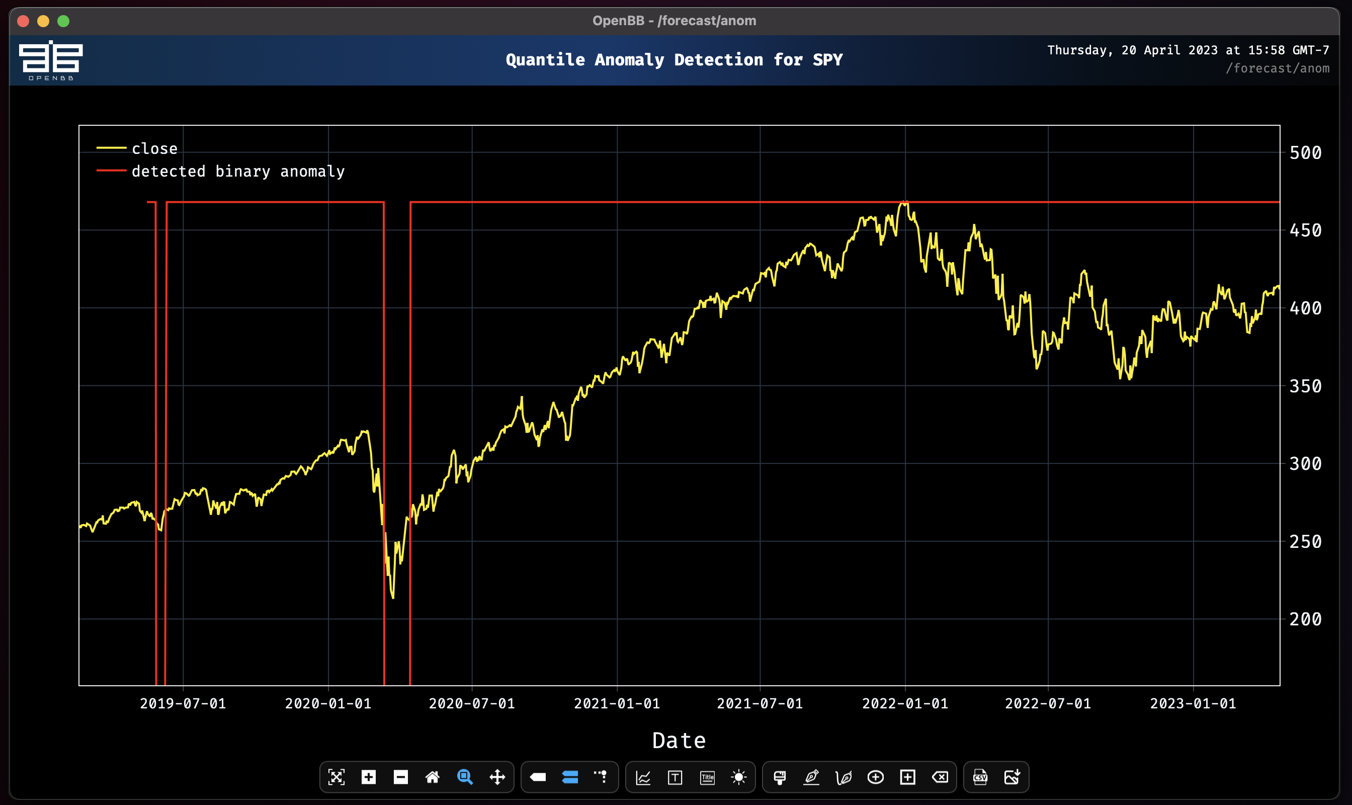
Quantile Anomaly Detection

anom performs a Quantile Anomaly detection on a given dataset. Read more about this calculation here.

anom -d SPY

Miscellaneous AI Tools

Whisper

The whisper feature allows users to transcribe, translate, and summarize videos on YouTube. These abilities empowers users to perform deeper research than ever before, and opens the door to a more complete view of the macroeconomic landscape. The models are not installed until the first time it is used, and they can be quite significant in size. Performance will vary, and there is currently not a method for offloading processing to dedicated GPUs.

whisper https://www.youtube.com/watch?v=G0Q0BtGQzrA

[DISCLAIMER]: This is a beta feature that uses standard NLP models. More recent models such as GPT will be added in future releases.

Downloading and Loading NLP Pipelines from cache...

All NLP Pipelines loaded.

Transcribing and summarizing...
Downloaded video "China stuck in 8 trillion dollar debt crisis | GyanJaraHatke with Sourabh Maheshwari". Generating subtitles...
Detected language: Hindi
100%|████████████████████████████████████████████████████████| 83567/83567 [04:25<00:00, 314.21frames/s]
100%|███████████████████████████████████████████████████████████████████| 11/11 [02:44<00:00, 14.99s/it]

-------------------------
Summary: Reduction: 81.38%
Sentiment: NEGATIVE: 73.2596
-------------------------
China is the largest economy in the world. Usually China's economy is seen in the global level of the economy of America...

A file with the transcript is saved to the OpenBBUserData folder.

Sample Workflow #1 (Beginner)

Let's begin by using one of the datasets we loaded in previously : SPY

We will be forecasting 5 Business days ahead for the remaider of these workflows unless specified.

Note: All models automatically perform Historical backtesting on the test split before providing a prediction.

We use MAPE for the default as it is quite convenient and scale independent since it calculates error as a percentage instead of an absolute value. There are many more metrics to compare time series. The metrics will compare only common slices of series when the two series are not aligned, and parallelize computation over a large number of pairs of series. Additional metrics to choose from are RMSE, MSE, and SMAPE.

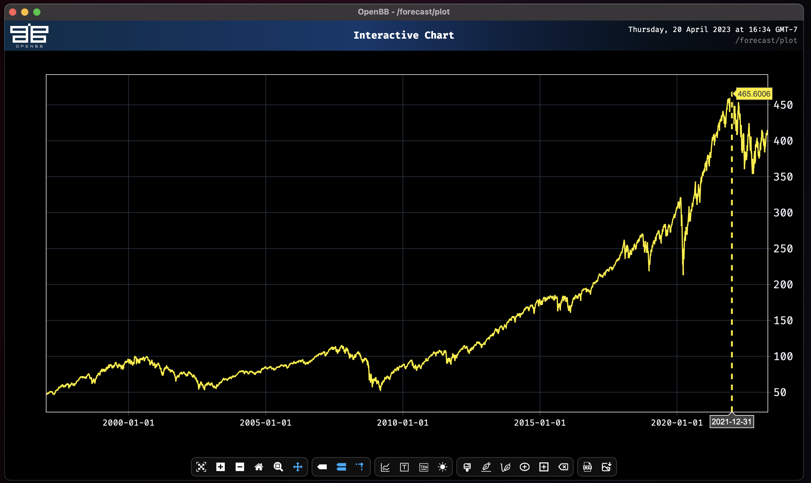
plot

plot SPY.close

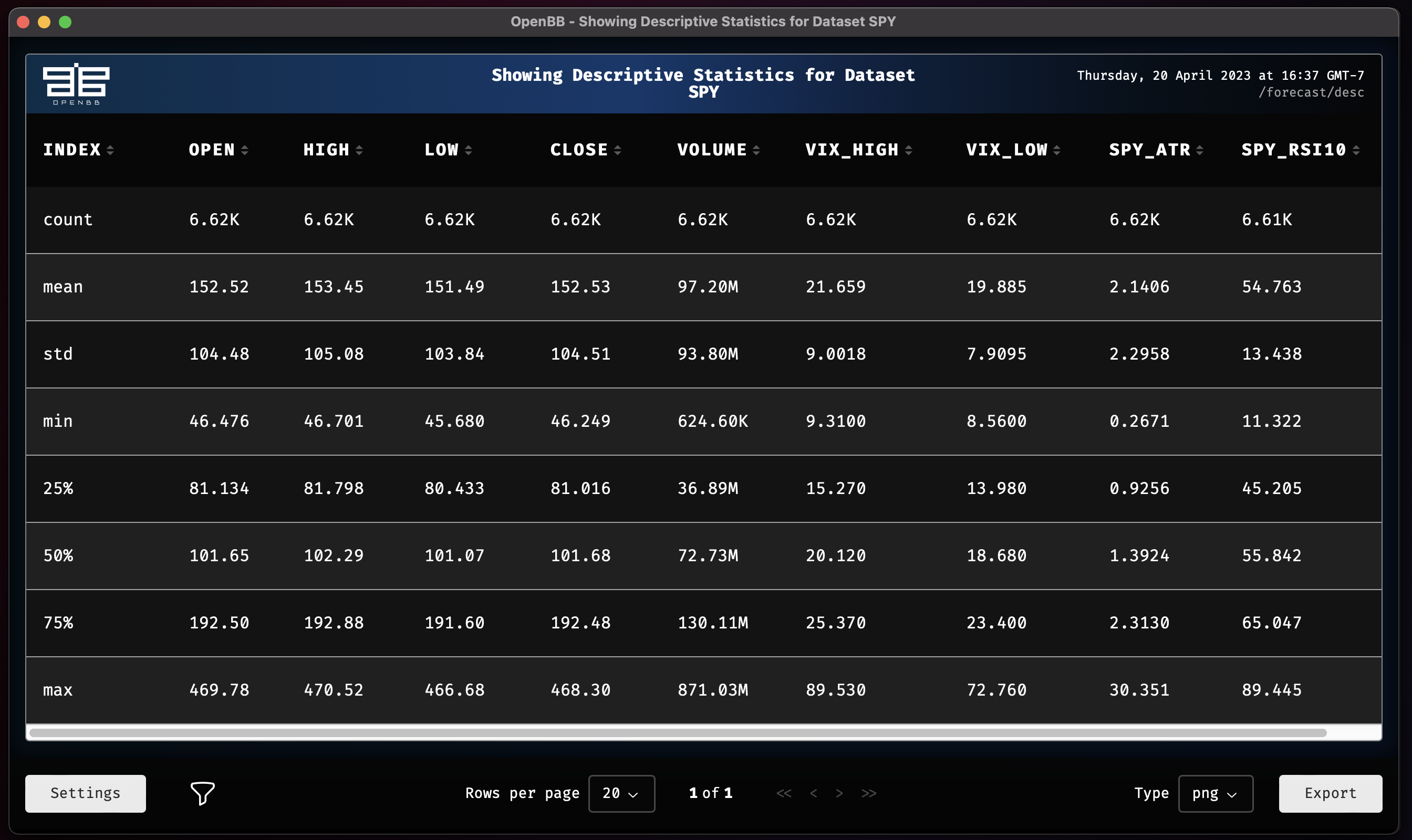
desc

desc SPY

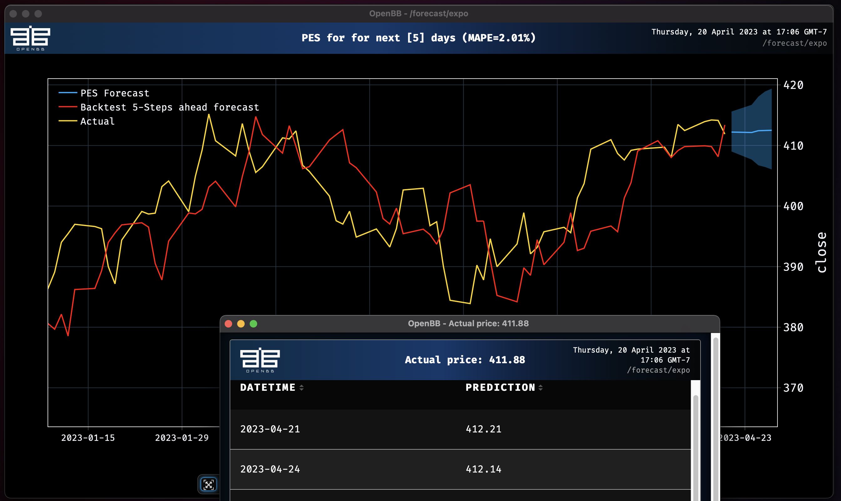
expo

Let's use a simple Probabilistic Exponential Smoothing Model to predict the close price. Keep in mind all models are performing automatic historical backtesting before providing future forecasts. Note that all models forecast close by default.

expo SPY

rnn

We can also play with some models that are bit more advanced. As we go down the list, models begin to become larger in parameter size and complexity. This will play a key role later on when we want to train models with past_covariates (aka. external factors).

This time lets test with a Recurrent Neural Network which by default uses an LSTM backbone. We can also choose to test out a GRU backbone to experiment. Let's do both and see if we can improve our accuracy and reduce the overall MAPE.

rnn SPY --forecast-only

Epoch 50: 100%|█████████████████████████████████████| 214/214 [00:02<00:00, 77.77it/s, loss=-4.31, v_num=logs, train_loss=-4.46, val_loss=-.985]

RNN model obtains MAPE: 3.13%

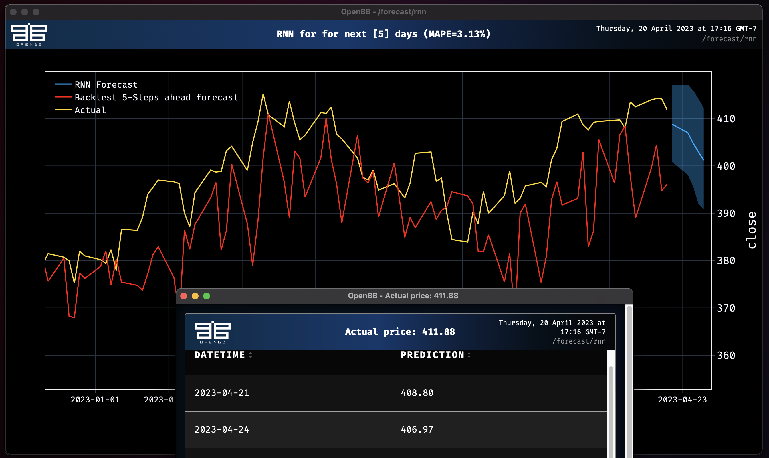
This result expresses a different view from the Probabilistic Exponential Smoothing Model.

For the second task, we would like to change the model type from LSTM --> GRU. Let's find out of this improves the MAPE score. Use the -h flag to understand the particular parameters one can change for RNN. (Please note that the parameters are different for each model).

rnn -h

usage: rnn [--hidden-dim HIDDEN_DIM] [--training_length TRAINING_LENGTH] [--naive] [-d {vix,SPY}] [-c TARGET_COLUMN] [-n N_DAYS]
           [-t TRAIN_SPLIT] [-i INPUT_CHUNK_LENGTH] [--force-reset FORCE_RESET] [--save-checkpoints SAVE_CHECKPOINTS]
           [--model-save-name MODEL_SAVE_NAME] [--n-epochs N_EPOCHS] [--model-type MODEL_TYPE] [--dropout DROPOUT] [--batch-size BATCH_SIZE]
           [--end S_END_DATE] [--start S_START_DATE] [--learning-rate LEARNING_RATE] [--residuals] [--forecast-only] [--export-pred-raw]
           [--metric {rmse,mse,mape,smape}] [-h] [--export EXPORT]

Perform RNN forecast (Vanilla RNN, LSTM, GRU): https://unit8co.github.io/darts/generated_api/darts.models.forecasting.rnn_model.html

options:
  --hidden-dim HIDDEN_DIM
                        Size for feature maps for each hidden RNN layer (h_n) (default: 20)
  --training_length TRAINING_LENGTH
                        The length of both input (target and covariates) and output (target) time series used during training. Generally
                        speaking, training_length should have a higher value than input_chunk_length because otherwise during training the RNN
                        is never run for as many iterations as it will during training. (default: 20)
  --naive               Show the naive baseline for a model. (default: False)
  -d {vix,SPY}, --dataset {vix,SPY}
                        The name of the dataset you want to select (default: None)
  -c TARGET_COLUMN, --target-column TARGET_COLUMN
                        The name of the specific column you want to use (default: close)
  -n N_DAYS, --n-days N_DAYS
                        prediction days. (default: 5)
  -t TRAIN_SPLIT, --train-split TRAIN_SPLIT
                        Start point for rolling training and forecast window. 0.0-1.0 (default: 0.85)
  -i INPUT_CHUNK_LENGTH, --input-chunk-length INPUT_CHUNK_LENGTH
                        Number of past time steps for forecasting module at prediction time. (default: 14)
  --force-reset FORCE_RESET
                        If set to True, any previously-existing model with the same name will be reset (all checkpoints will be discarded).
                        (default: True)
  --save-checkpoints SAVE_CHECKPOINTS
                        Whether to automatically save the untrained model and checkpoints. (default: True)
  --model-save-name MODEL_SAVE_NAME
                        Name of the model to save. (default: rnn_model)
  --n-epochs N_EPOCHS   Number of epochs over which to train the model. (default: 300)
  --model-type MODEL_TYPE
                        Enter a string specifying the RNN module type ("RNN", "LSTM" or "GRU") (default: LSTM)
  --dropout DROPOUT     Fraction of neurons affected by Dropout, from 0 to 1. (default: 0)
  --batch-size BATCH_SIZE
                        Number of time series (input and output) used in each training pass (default: 32)
  --end S_END_DATE      The end date (format YYYY-MM-DD) to select for testing (default: None)
  --start S_START_DATE  The start date (format YYYY-MM-DD) to select for testing (default: None)
  --learning-rate LEARNING_RATE
                        Learning rate during training. (default: 0.001)
  --residuals           Show the residuals for the model. (default: False)
  --forecast-only       Do not plot the historical data without forecasts. (default: False)
  --export-pred-raw     Export predictions to a csv file. (default: False)
  --metric {rmse,mse,mape,smape}
                        Calculate precision based on a specific metric (rmse, mse, mape) (default: mape)
  -h, --help            show this help message (default: False)
  --export EXPORT       Export figure into png, jpg, pdf, svg (default: )

For more information and examples, use 'about rnn' to access the related guide.

Lets change the --model-type parameter to GRU and rerun.

rnn SPY --model-type GRU --forecast-only

Epoch 85: 100%|█████████████████████████████████████| 214/214 [00:02<00:00, 75.10it/s, loss=-4.45, v_num=logs, train_loss=-4.35, val_loss=-2.35]

RNN model obtains MAPE: 2.77%

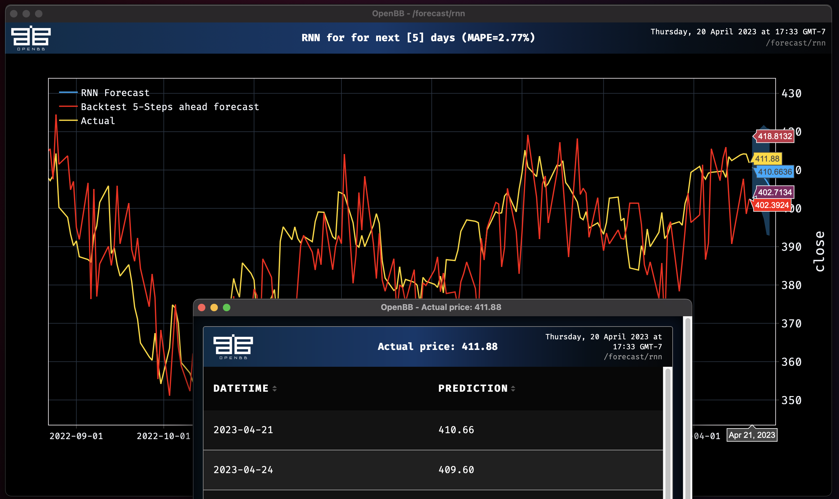
We improved the accuracy score, great work!

note

The take away for this is that all models should work out of the box when forecasting for a particular time series. One can switch the target by specifying a -c for TARGET_COLUMN and test out performance with multiple different models with a single command.

Sample Workflow #2 (Advanced)

To build successful models and improve accuracy over time, it is important to capture external data related to the time series you are training on. This can be seen in everyday applications:

• Observed rainfalls and known weather forecasts can help to predict hydro and solar electricity production
• Recently-observed activity on an e-commerce website can help predict future sales.
• Making the model aware of up-coming holidays can help sales forecasting.

In fact, more often than not, strictly relying on the history of a time series to predict its future is missing a lot of valuable information.

Past covariates are time series whose past values are known at prediction time. Those series often contain values that have to be observed to be known.

To explore this topic more, please read the blog post written by the authors of Darts.

Note that only the following models can handle past_covariates: BlockRNNModel, NBEATSModel, TCNModel, TransformerModel, RegressionModel (incl. LinearRegressionModel), Temporal Fusion Transformer

Earlier on in the guide we managed to accomplish the following:

• Load multiple datasets.
• Combine datasets.
• Rename columns.
• Delete columns.

We will continue this workflow by:

• Adding some correlation analysis.
• Train models with past_covariates.

For practice, let's start fresh and rebuild the same dataset. The OpenBB Routine Scripts can make quick work out of this chore. Copy the block below and create a new .openbb file, in ~/OpenBBUserData/routines/, to follow along.

/stocks
load SPY --start 1997-01-01
forecast
..
load ^VIX --start 1997-01-01
forecast
combine --dataset SPY -c ^VIX.high
combine --dataset SPY -c ^VIX.low
delete --delete SPY.adj_close
delete --delete SPY.stock_splits
delete --delete SPY.dividends
atr -d SPY
rsi -d SPY
rename -d SPY --oldcol RSI_10_close --newcol SPY_rsi10
rename -d SPY --oldcol true_range --newcol SPY_atr
show SPY

Restart the Terminal to ensure that the routine file is found by the /exe command, and then run it.

exe --file forecast_demo.openbb

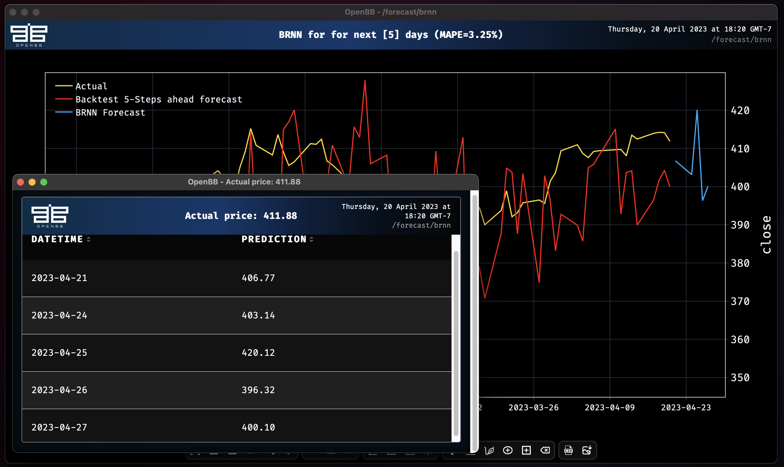
brnn

Now take the new dataset and train a simple Block RNN model on SPY's close price, and again using past_covariates on a single column.

Without past covariates:

brnn SPY --forecast-only

Epoch 196: 100%|███████████████████████████████████| 214/214 [00:01<00:00, 107.42it/s, loss=-4.09, v_num=logs, train_loss=-4.07, val_loss=-1.53]

Block RNN model obtains MAPE: 3.25%

With covariates:

To use any covariates, there are two options:

• specify specific columns with --past-covariates
• specify all columns as past covariates except the one you are forecasting --all-past-covariates

brnn SPY --forecast-only --past-covariates volume

Covariate #0: volume
Epoch 86: 100%|████████████████████████████████████████| 214/214 [00:02<00:00, 74.77it/s, loss=-4, v_num=logs, train_loss=-4.19, val_loss=-1.53]
Block RNN model obtains MAPE: 4.69%

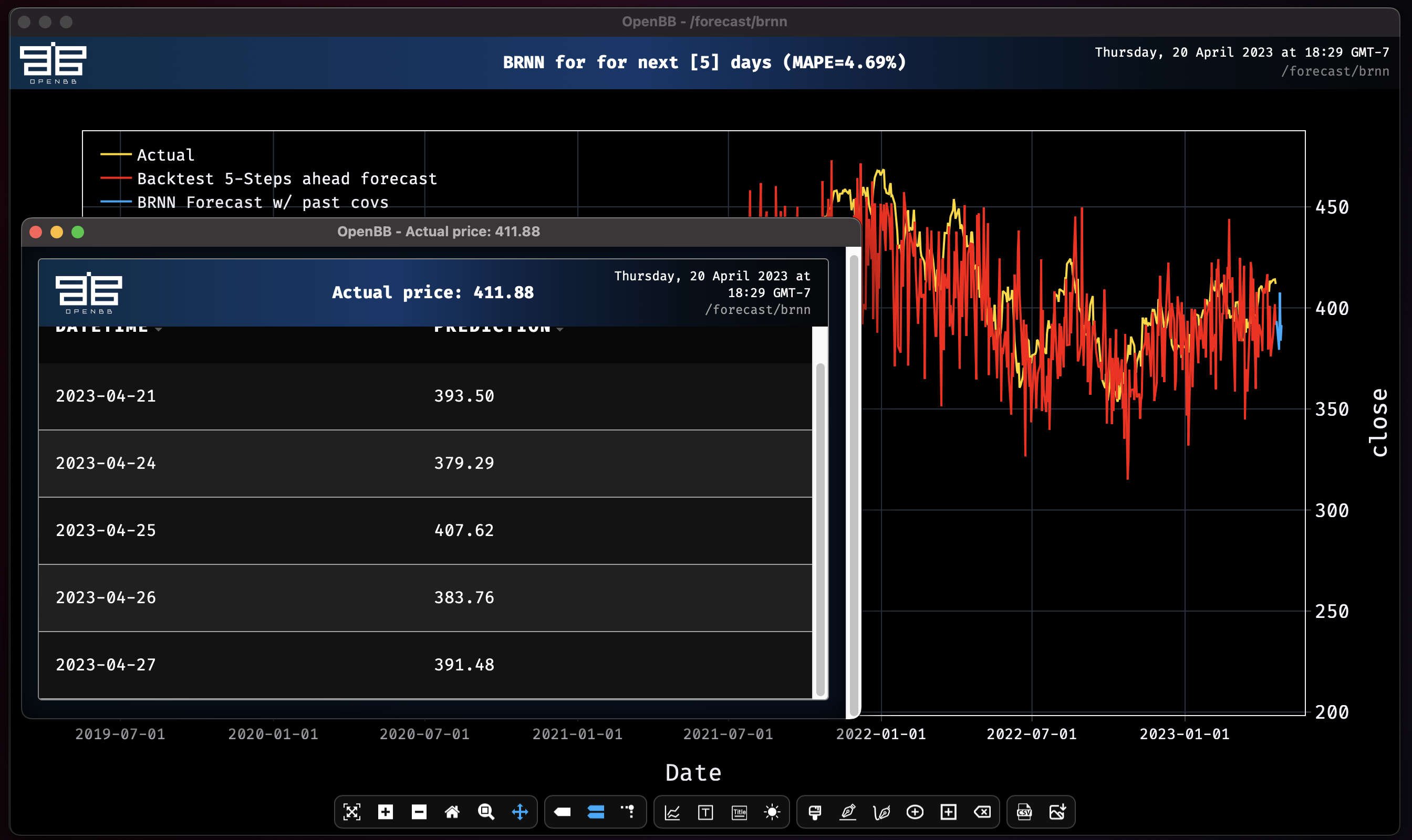
It is evident here that adding in the external variable of volume negatively affected the accuracy.

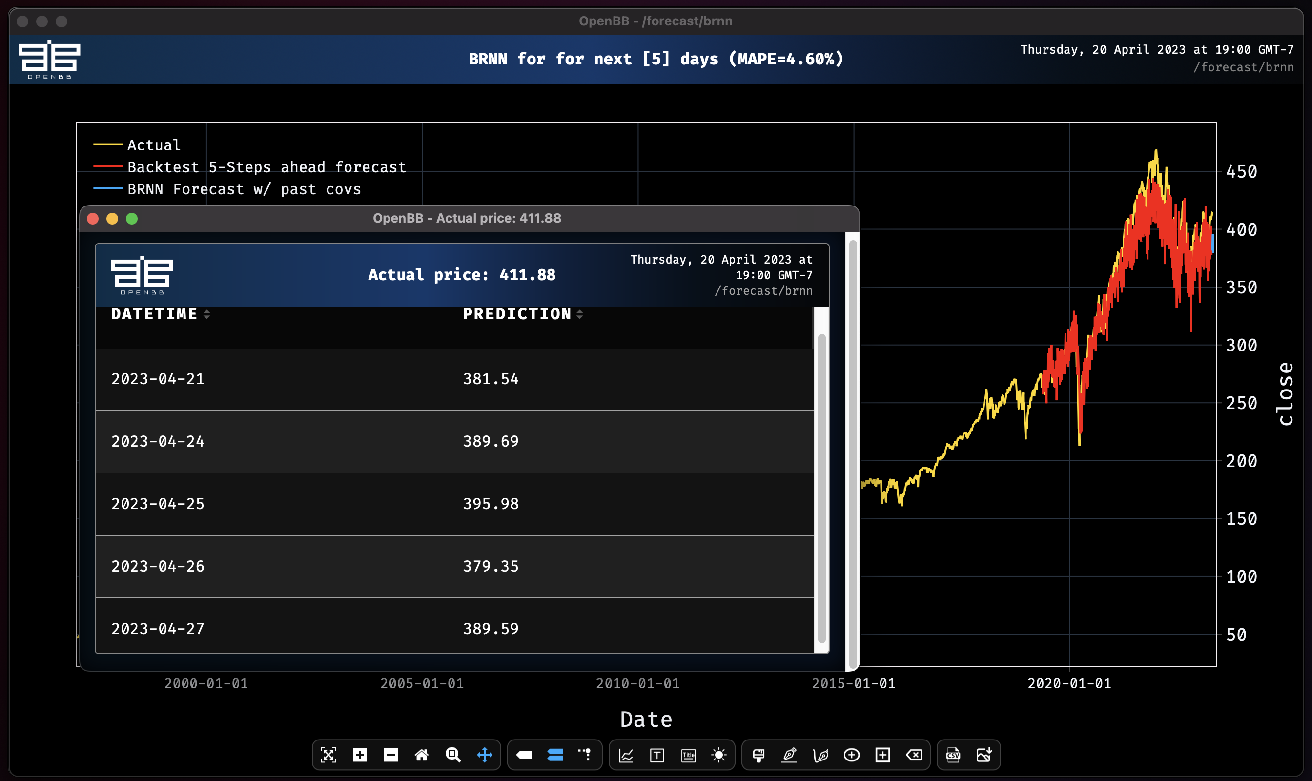
Let's try adding a new column for the 200-day moving average.

ema -d SPY --period 200/brnn -d SPY --past-covariates EMA_200

Successfully added 'EMA_200' to 'SPY' dataset
Covariate #0: EMA_200
Epoch 79: 100%|█████████████████████████████████████| 214/214 [00:02<00:00, 87.78it/s, loss=-3.81, v_num=logs, train_loss=-3.78, val_loss=-.435
Block RNN model obtains MAPE: 4.60%

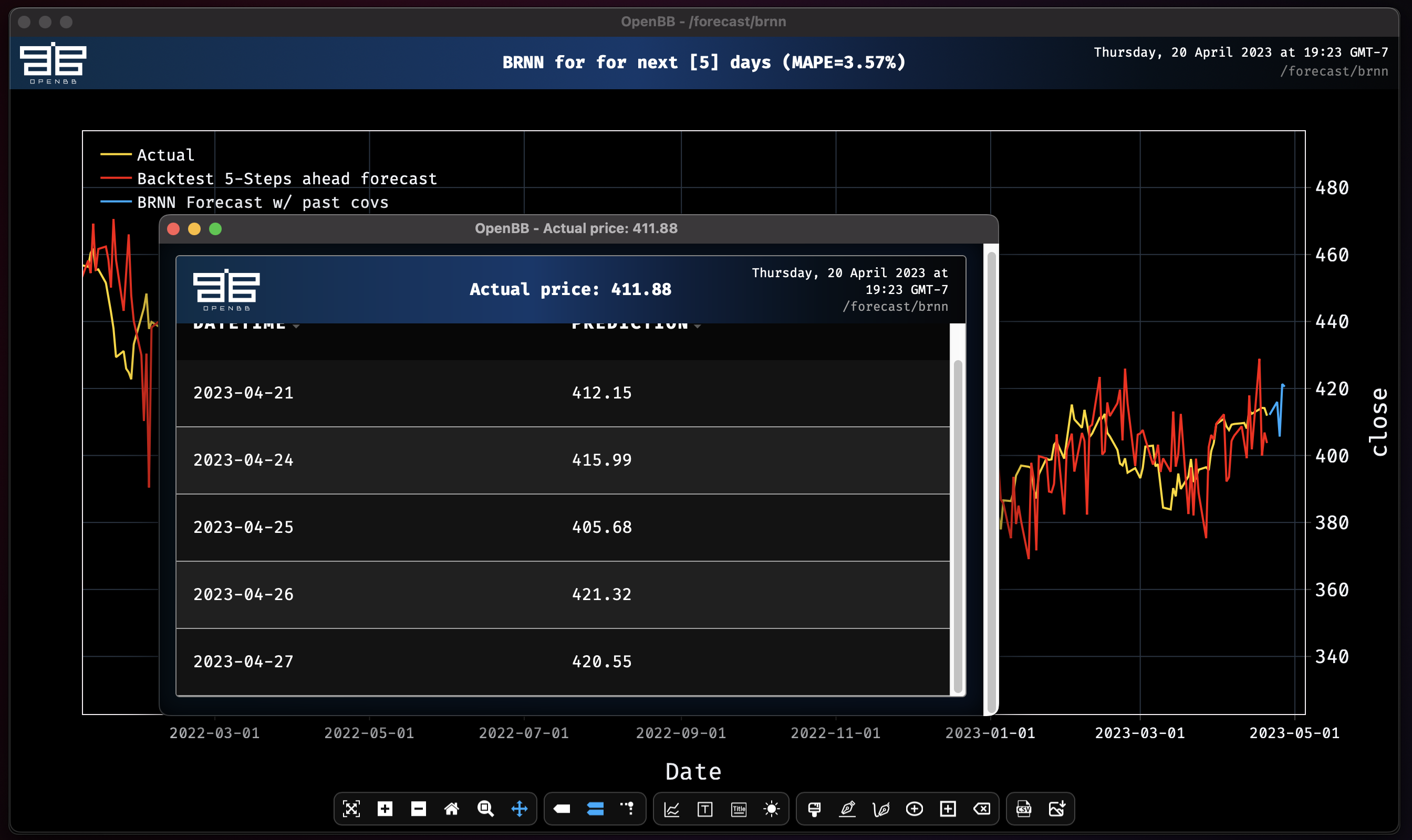
This isn't an improvement. It's possible that there is too much noise in the data, so let's try shortening the length of time being used to train.

brnn -d SPY --past-covariates EMA_200 -t 0.95

Covariate #0: EMA_200
Epoch 87: 100%|█████████████████████████████████████| 215/215 [00:02<00:00, 82.81it/s, loss=-3.87, v_num=logs, train_loss=-4.29, val_loss=-1.59]
Block RNN model obtains MAPE: 3.38%

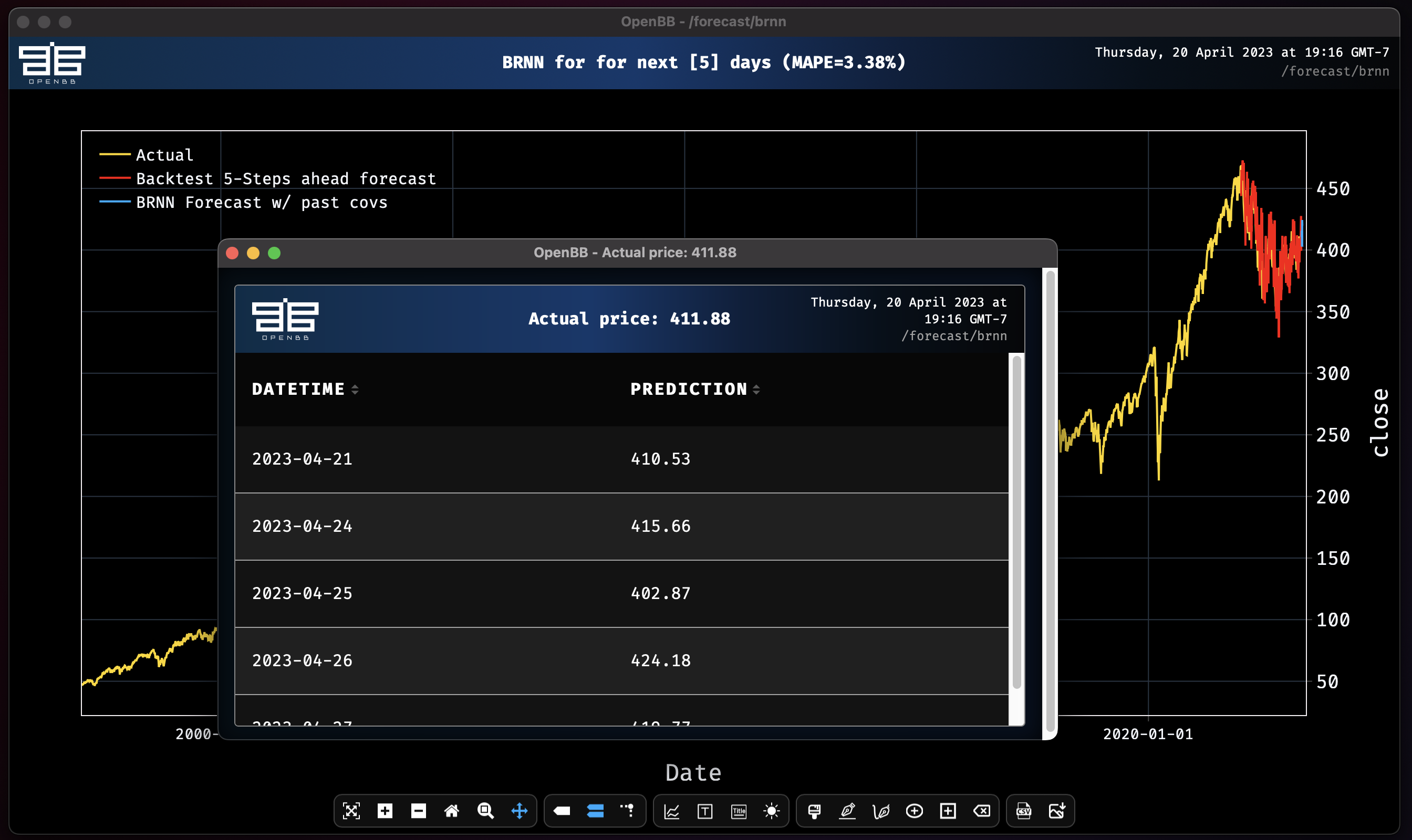
Removing the 2020 volatility from the window of observation made a massive improvement to the forecast. Now let's see add all the columns in the dataset as past covariates.

brnn -d SPY --all-past-covariates -t 0.95

Covariate #0: open
Covariate #1: high
Covariate #2: low
Covariate #3: volume
Covariate #4: ^VIX_high
Covariate #5: ^VIX_low
Covariate #6: SPY_atr
Covariate #7: SPY_rsi10
Covariate #8: EMA_200
Epoch 39: 100%|█████████████████████████████████████| 215/215 [00:02<00:00, 83.50it/s, loss=-3.92, v_num=logs, train_loss=-4.03, val_loss=-2.14]
Block RNN model obtains MAPE: 3.57%

Adding all of the columns that were created doesn't improve the MAPE score, but it does narrow the range of forecasted prices. Playing around like this shows how small changes can have a large impact on a forecast. It is important to test many variables and parameters without getting too caught up overfitting any particular model. Validate a thesis before dedicating a large amount of time into it.

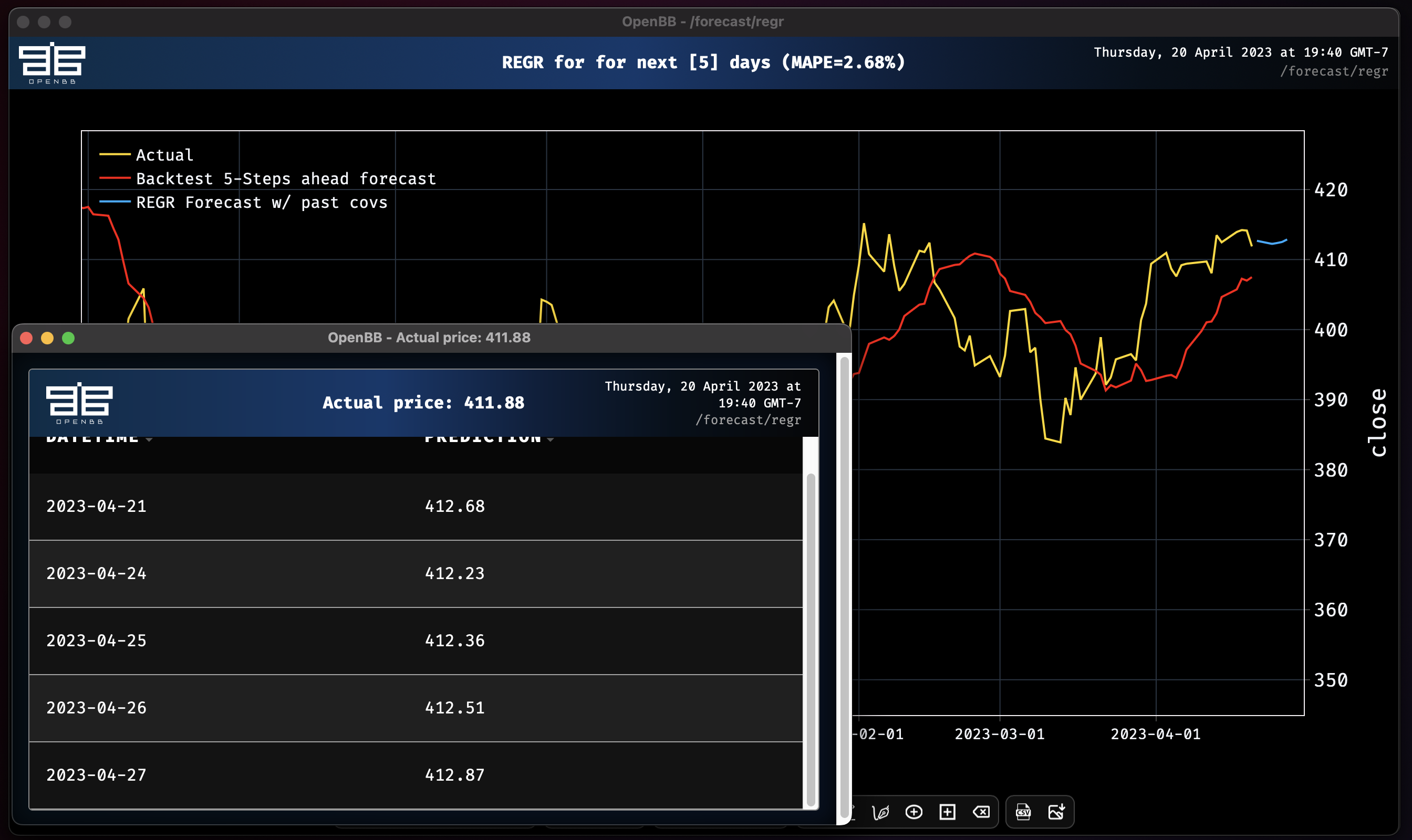
regr

Using the regr function with all-past-covariates on the same dataset gives dramatically different forecast.

regr SPY --all-past-covariates

Covariate #0: open
Covariate #1: high
Covariate #2: low
Covariate #3: volume
Covariate #4: ^VIX_high
Covariate #5: ^VIX_low
Covariate #6: SPY_atr
Covariate #7: SPY_rsi10
Predicting Regression for 5 days
100%|███████████████████████████████████████████████████████████████████████████████████████████████████████| 1026/1026 [00:48<00:00, 21.35it/s]
Regression model obtains MAPE: 2.68%

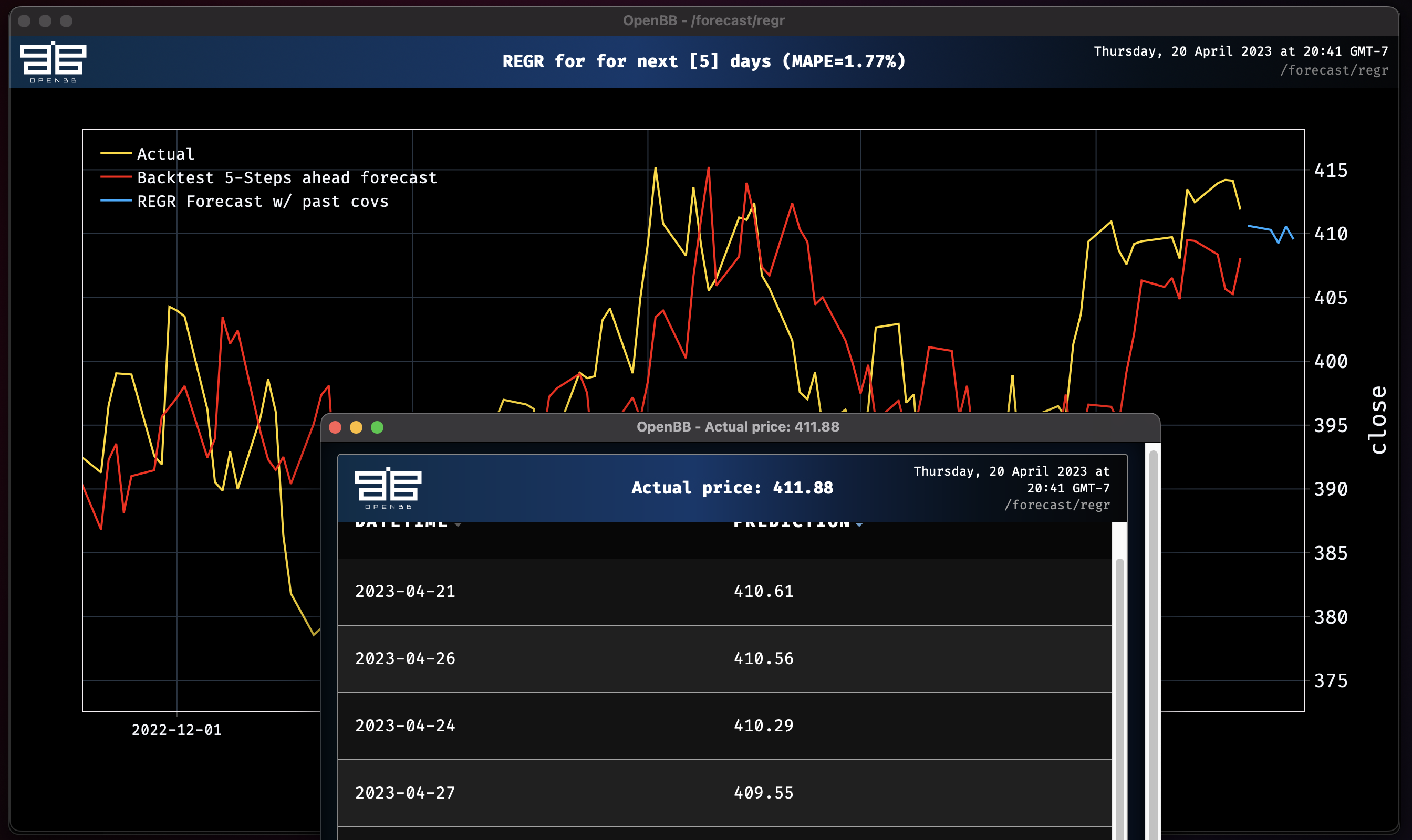
Now that we know how to use covariates, and are starting to understand their effects, let's examine the impact of MSFT and AAPL closing prices on the regression forecast for SPY. We will discard the previous work and start fresh.

The cache can be purged by resetting the Terminal. Use this command to clear it:

/r

Now we will fetch the data and combine the columns:

/stocks/load spy
forecast
..
load aapl
forecast
..
load msft
forecast
delete --delete SPY.stock_splits
delete --delete SPY.adj_close
delete --delete SPY.dividends
combine SPY -c AAPL.close
combine SPY -c MSFT.close
regr SPY --forecast-only --past-covariates AAPL_close,MSFT_close

Remember: You can use unlimited number of past_covariates but they must all be combined into a single dataframe with the target forecast time series before training.

Covariate #0: AAPL_close
Covariate #1: MSFT_close
Predicting Regression for 5 days
100%|█████████████████████████████████████████████████████████████████████████████████████████████████████████| 115/115 [00:01<00:00, 96.07it/s]
Regression model obtains MAPE: 1.77%

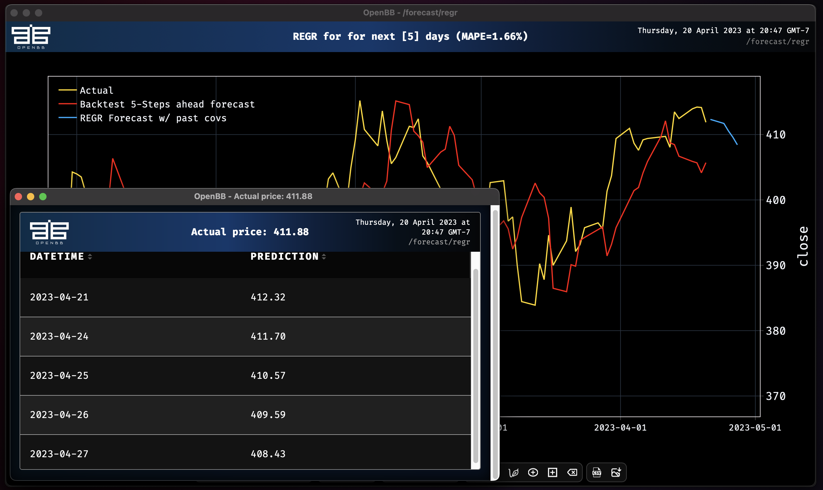
Adding the rest of the columns as past covariates improves the MAPE score slightly and starts to take a more directional view.

regr --all-past-covariates -d SPY

Covariate #0: open
Covariate #1: high
Covariate #2: low
Covariate #3: volume
Covariate #4: AAPL_close
Covariate #5: MSFT_close
Predicting Regression for 5 days
100%|████████████████████████████████████████████████████████████████████████████████████████████████████████| 115/115 [00:00<00:00, 117.16it/s]
Regression model obtains MAPE: 1.66%

note

The examples here are over-simplified as a means for demonstrating a framework to create and conduct experiments. It is important to keep in mind that these are tools, they are not oracles, and that results may vary. If you have any questions, requests for new feature engineering and model additions, or just want to be part of the conversation, please join us on Discord. Happy hacking!