Quantitative Analysis

The qa module is the Terminal's Quantitative Analysis menu for the SDK environment. It provides users with more ways to interact with the library of functions, and provides cross-disciplinary utility. To activate the code completion for the menu, enter . after, openbb.qa.

How to Use

The functions of the qa module are grouped into categories, listed below along with a short description.

Path	Type	Description
openbb.qa.acf	Plot	Plots Auto and Partial Correlation of Returns and Change in Returns
openbb.qa.bw	Plot	Box and Whisker Plot
openbb.qa.calculate_adjusted_var	Risk	Calculates VaR, adjusted for skew and kurtosis (Cornish-Fisher-Expansion)
openbb.qa.cdf	Plot	Plots the Cumulative Distribution Function
openbb.qa.cusum	Plot	Plots the Cumulative Sum Algorithm
openbb.qa.decompose	Plot	Decomposition in Cyclic-Trend, Season & Residuals of Prices
openbb.qa.es	Statistics	Expected Shortfall per percentile
openbb.qa.kurtosis	Rolling Metrics	Rolling Kurtosis of Distribution of Prices
openbb.qa.line	Plot	Customizable Line Plot, With Annotations
openbb.qa.normality	Statistics	Normality Statistics and Tests
openbb.qa.omega	Risk	Omega Ratio (Risk/Return Performance Measure)
openbb.qa.quantile	Rolling Metrics	Rolling Median and Quantile of Prices
openbb.qa.qqplot	Plot	QQ Plot for Data Against Normal Quantiles
openbb.qa.rolling	Rolling Metrics	Rolling Mean and Standard Deviation of Prices
openbb.qa.sharpe	Risk	Sharpe Ratio (Measure of Risk-Adjusted Return)
openbb.qa.skew	Rolling Metrics	Rolling Skewness of Distribution of Prices
openbb.qa.sortino	Risk	Sortino Ratio Risk Adjustment Metric
openbb.qa.spread	Rolling Metrics	Rolling Variance and Standard Deviation of Prices
openbb.qa.summary	Statistics	A Brief Summary of Statistics for the DataFrame
openbb.qa.unitroot	Statistics	Normality Statistics and Tests
openbb.qa.var	Risk	Value at Risk

Examples

Import Statements

The examples below will assume that the following statements are included in the first block of code:

import quandl
import pandas as pd
from openbb_terminal.sdk import openbb
from openbb_terminal import config_terminal as cfg

# %matplotlib inline (uncomment if using a Jupyter environment)

Get Data

This example collects data from Nasdaq Data Link, and requires registering for a free API key. Qunadl is the Python client for the Nasdaq Data Link API.

shiller_pe_rdiff = quandl.get('MULTPL/SHILLER_PE_RATIO_MONTH', collapse = 'monthly', transform = 'rdiff', api_key = cfg.API_KEY_QUANDL)
shiller_pe_rdiff.rename(columns={'Value':'P/E % Change'}, inplace = True)
shiller_pe_ratio = quandl.get('MULTPL/SHILLER_PE_RATIO_MONTH', collapse = 'monthly', api_key = cfg.API_KEY_QUANDL)
shiller_pe_ratio.rename(columns={'Value':'P/E Ratio'}, inplace = True)

sp500_inf_adj = quandl.get('MULTPL/SP500_INFLADJ_MONTH', collapse = 'monthly', api_key = cfg.API_KEY_QUANDL)
sp500_inf_adj.rename(columns = {'Value': 'S&P Inflation-Adjusted Value'}, inplace = True)
sp500_inf_adj_rdiff = quandl.get('MULTPL/SP500_INFLADJ_MONTH', collapse = 'monthly', transform = 'rdiff', api_key = cfg.API_KEY_QUANDL)
sp500_inf_adj_rdiff.rename(columns = {'Value':'S&P 500 % Change'}, inplace = True)

shiller_pe = shiller_pe_ratio.join(shiller_pe_rdiff)
sp500_inf_adj = sp500_inf_adj.join(sp500_inf_adj_rdiff)

sp500_df = sp500_inf_adj.join(shiller_pe)

sp500_df

Date	S&P Inflation-Adjusted Value	S&P 500 % Change	P/E Ratio	P/E % Change
2022-08-31 00:00:00	3955	0.0092504	29.64	0.022069
2022-09-30 00:00:00	3585.62	-0.0933957	26.84	-0.0944669
2022-10-31 00:00:00	3871.98	0.0798635	28.53	0.0629657
2022-11-30 00:00:00	3856.1	-0.00410126	28.37	-0.00560813

This particular data series contains 150 years of monthly values. It is among the longest uninterrupted timeseries available in the public domain, and it is cited frequently in macroeconomic research.

Summary

Get a summary of statistics for each column with qa.summary:

openbb.qa.summary(sp500_df)

	S&P Inflation-Adjusted Value	S&P 500 % Change	P/E Ratio	P/E % Change
count	1823	1822	1822	1821
mean	697.396	0.0028703	16.9914	0.00137084
std	834.501	0.0424378	7.07094	0.0412196
min	80.31	-0.264738	4.78	-0.268992
10%	152.404	-0.0447494	9.31	-0.0449735
25%	203.47	-0.0172803	11.7	-0.0183028
50%	309.83	0.00553122	15.895	0.00446999
75%	778.42	0.0260009	20.5575	0.0246575
90%	1907.87	0.04505	26.467	0.0426357
max	4786.79	0.514085	44.19	0.511986
var	696392	0.00180097	49.9982	0.00169906

Spread

Add the variance and standard deviation, over a specified window (three-months), to the DataFrame:

std,variance = openbb.qa.spread(data = sp500_df['S&P 500 % Change'], window = 3)
std.rename(columns = {'STDEV_3':'Three-Month Standard Deviation'}, inplace = True)
variance.rename(columns = {'VAR_3': 'Three-Month Variance'}, inplace =True)
sp500_df = sp500_df.join([std,variance])
sp500_df.rename_axis('date', inplace = True)
sp500_df.tail(2)

date	S&P Inflation-Adjusted Value	S&P 500 % Change	P/E Ratio	P/E % Change	Three-Month Standard Deviation	Three-Month Variance
2022-10-31 00:00:00	3871.98	0.0798635	28.53	0.0629657	0.0871217	0.00759019
2022-11-30 00:00:00	3856.1	-0.00410126	28.37	-0.00560813	0.0866432	0.00750705

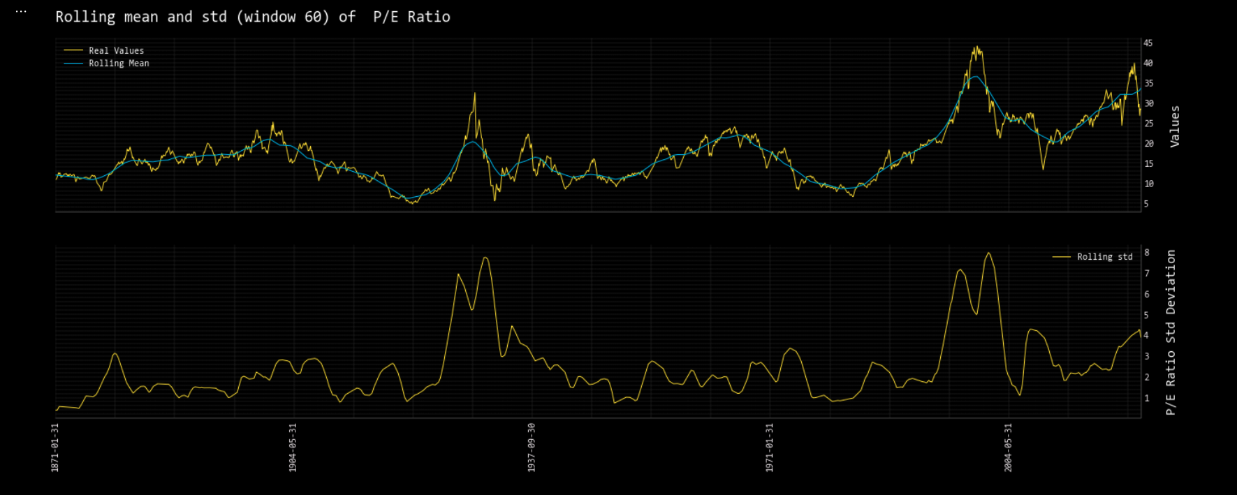
The rolling mean average and standard deviation is calculated with the rolling command. Adding, _chart, to this will return an inline chart within a Jupyter Notebook. For the example below, window, 60, represents a five-year period.

Rolling

openbb.qa.rolling_chart(sp500_df, target = 'P/E Ratio', window = 60, symbol = '')

Unit Root Test

Perform a unit root test with unitroot:

help(openbb.qa.unitroot)

        Parameters
        ----------
        data : pd.DataFrame
            DataFrame of target variable
        fuller_reg : str
            Type of regression of ADF test. Can be ‘c’,’ct’,’ctt’,’nc’ 'c' - Constant and t - trend order
        kpss_reg : str
            Type of regression for KPSS test.  Can be ‘c’,’ct'

        Returns
        -------
        pd.DataFrame
            Dataframe with results of ADF test and KPSS test

openbb.qa.unitroot(sp500_df['P/E % Change'])

	ADF	KPSS
Test Statistic	-10.7075	0.34061374135067696
P-Value	3.3972e-19	0.1
NLags	20	2
Nobs	1800
ICBest	-6491.14