Forecast

The Forecast module provides programmatic access to the same commands found in the OpenBB Terminal Forecast menu. The extensive library of models, built on top of the u8darts library, are easily tuned with hyper-parameters.

How to Use

The Forecast menu was designed specifically for the CLI application, and consequently, the operation of these commands do not mirror the workflow of the OpenBB Terminal. This will be improved in the future to more closely resemble it, and this guide will highlight some notable differences.

Commands within the forecast module are representatives from three broad categories:

Exploration
Feature Engineering
Model

Each command is listed below with a short description. A majority of functions will also have an additional syntax, _chart, for displaying the generated charts inline. For ease of use, we recommend using the _chart version for Model functions.

Path	Type	Description
openbb.forecast.atr	Feature Engineering	Add a Column for the Average True Range
openbb.forecast.autoces	Model	Automatic Complex Exponential Smoothing Model
openbb.forecast.autoets	Model	Automatic ETS (Error, Trend, Seasonality) Model
openbb.forecast.autoselect	Model	Automatically Selects the Best Statistical Model From AutoARIMA, AutoETS, AutoCES, MSTL, etc.
openbb.forecast.brnn	Model	Block Recurrent Neural Network (RNN, LSTM, GRU) (feat. Past covariates)
openbb.forecast.clean	Exploration	Fill or Drop NaN Values
openbb.forecast.combine	Exploration	Combine Columns From Different Datasets
openbb.forecast.corr	Exploration	Correlation Coefficients Between Columns of a Dataset
openbb.forecast.delete	Exploration	Delete Columns From a Dataset
openbb.forecast.delta	Feature Engineering	Add a Column for % Change
openbb.forecast.desc	Exploration	Show Descriptive Statistics for a Dataset
openbb.forecast.ema	Feature Engineering	Add a Column for Exponentially Weighted Moving Average
openbb.forecast.expo	Model	Probabilistic Exponential Smoothing
openbb.forecast.export	Export	Export a Processed Dataset as a CSV or XLSX File
openbb.forecast.linregr	Model	Probabilistic Linear Regression (feat. Past covariates and Explainability)
openbb.forecast.load	Import	Import a Local CSV or XLSX File
openbb.forecast.mom	Feature Engineering	Add a Column for Momentum
openbb.forecast.nbeats	Model	Neural Bayesian Estimation (feat. Past covariates)
openbb.forecast.nhits	Model	Neural Hierarchical Interpolation (feat. Past covariates)
openbb.forecast.plot	Exploration	Plots Specific Columns From a Loaded Dataset
openbb.forecast.regr	Model	Regression (feat. Past covariates and Explainability)
openbb.forecast.rename	Exploration	Rename Columns in a Dataset
openbb.forecast.rnn	Model	Probabilistic Recurrent Neural Network (RNN, LSTM, GRU)
openbb.forecast.roc	Feature Engineering	Add a Column for Rate of Change
openbb.forecast.rsi	Feature Engineering	Add a Column for Relative Strength Index
openbb.forecast.rwd	Model	Random Walk with Drift Model
openbb.forecast.season	Exploration	Plot Seasonality of a Column in a Dataset
openbb.forecast.seasonalnaive	Model	Seasonal Naive Model
openbb.forecast.signal	Feature Engineering	Add a Column for Price Signal (Short vs. Long Term)
openbb.forecast.sto	Feature Engineering	Add a Column for Stochastic Oscillator %K and %D
openbb.forecast.tcn	Model	Temporal Convolutional Neural Network (feat. Past covariates)
openbb.forecast.tft	Model	Temporal Fusion Transformer Network(feat. Past covariates)
openbb.forecast.theta	Model	Theta Method
openbb.forecast.trans	Model	Transformer Network (feat. Past covariates)

Alternatively, the contents of the menu is printed with:

help(openbb.forecast)

Type hints and code completion will be activated upon entering the ., after, openbb.forecast. The first step is always going to involve loading some data. Let's walk through a procedure for procuring a DataFrame with some examples below.

Examples

Import Statements

The examples provided below will assume that the following import block is included at the beginning of the Python script or Notebook file:

from openbb_terminal.sdk import openbb
import pandas as pd
# %matplotlib inline (uncomment if using a Jupyter Interactive Terminal or Notebook)

Loading Data

This library of models are specifically for time-series, and consequently, the data must follow some formatting guidelines:

If the index is not a date, it must be sequentially ordered and evenly spaced - i.e., it can't be indexed like: [1,2,5,11,50]
A datetime index must be spaced evenly - i.e., monthly data is better handled when the interval date is the first of the month.
If the datetime index is a weekly interval, use a Monday-Friday format.
Intraday data is not officially supported at this time.

The equities market revolves around the S&P 500, so let's take a look at the ETF, SPY, from inception:

spy = openbb.stocks.load('SPY', start_date = '1990-01-01')

Loading Daily data for SPY with starting period 1993-01-29.

The printed message indicates that the first day of available data is not the same as the requested start date. Wikipedia shows the fund was launched on January 22, 1993. The product was marketed and sold to liquidity providers prior to trading on a public exchange, so this DataFrame is pretty darn close to the inception date. We can confirm that this data arrived as expected by printing the created DataFrame.

spy.head(5)

date	Open	High	Low	Close	Adj Close	Volume
1993-01-29 00:00:00	43.9688	43.9688	43.75	43.9375	25.334	1.0032e+06
1993-02-01 00:00:00	43.9688	44.25	43.9688	44.25	25.5142	480500
1993-02-02 00:00:00	44.2188	44.375	44.125	44.3438	25.5683	201300
1993-02-03 00:00:00	44.4062	44.8438	44.375	44.8125	25.8385	529400
1993-02-04 00:00:00	44.9688	45.0938	44.4688	45	25.9467	531500

Plot

The data can also be inspected visually, openbb.forecast.plot:

openbb.forecast.plot(data=spy, columns = ['Adj Close'])

openbb.forecast.plot

Theta

Data consisting of a numeric value and a datetime index is sufficient enough for feeding the inputs to a forecast model. One important distinction between the Terminal and SDK is that the target_column must be explicitly declared when using the SDK, if it is not labeled as "close". It is case-sensitive.

To use a forecast model with default parameters, all that is required in the syntax is:

The name of the dataset.
The target column for the forecast.

A basic, default, syntax will look like:

openbb.forecast.theta_chart(data = spy, target_column = 'Adj Close')

The default number of days to predict for all models is five. If the interval of the time-series is not daily, days equates to the interval of the index.

Theta Model obtains MAPE: 1.91%

openbb.forecast.theta_chart

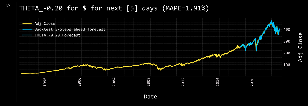
Datetime	Prediction
2022-11-24	402.62
2022-11-25	402.92
2022-11-28	403.14
2022-11-29	403.38
2022-11-30	403.59

Refer to the docstrings to learn about each model's unique set of arguments.

help(openbb.forecast.theta_chart)

Feature Engineering

This category of functions are for adding columns to a dataset that are the results of calculations, like technical and quantitative analysis. Individual parameters will vary slightly between functions, but syntax construction will be similar.

EMA

A moving average provides an indication of the trend of the price movement by cutting down the amount of "noise" in a price chart.

help(openbb.forecast.ema)

    Parameters
    ----------
    dataset : pd.DataFrame
        The dataset you wish to clean
    target_column : str
        The column you wish to add the EMA to
    period : int
        Time Span

    Returns
    -------
    pd.DataFrame
        Dataframe with added EMA column

The example below adds a column to the spy dataset for the 150-day exponential moving average of the adjusted-close price.

spy = openbb.forecast.ema(spy, target_column = 'Adj Close', period = 150)

spy.tail(3)

	date	Open	High	Low	Close	Adj Close	Volume	EMA_150
7508	2022-11-21	394.64	395.82	392.66	394.59	394.59	51243200	394.923
7509	2022-11-22	396.63	400.07	395.15	399.9	399.9	60429000	394.989
7510	2022-11-23	399.55	402.93	399.31	402.42	402.42	68161400	395.087

Additional columns can be added for each desired period length of the calculation:

spy = openbb.forecast.ema(spy, target_column = 'Adj Close', period = 20)

spy.tail(3)

	date	Open	High	Low	Close	Adj Close	Volume	EMA_150	EMA_20
7508	2022-11-21	394.64	395.82	392.66	394.59	394.59	51243200	394.923	387.237
7509	2022-11-22	396.63	400.07	395.15	399.9	399.9	60429000	394.989	388.443
7510	2022-11-23	399.55	402.93	399.31	402.42	402.42	68161400	395.087	389.775

The process can be repeated as required.

RSI

Similar to ema, rsi adds a column for the Relative Strength Index. The three variables are the same here as above. A period of ten equates to ten trading days, or two-weeks.

spy = openbb.forecast.rsi(spy, target_column = 'Adj Close', period = 10)

spy.tail(3)

	date	Open	High	Low	Close	Adj Close	Volume	EMA_150	EMA_20	RSI_10_Adj Close
7508	2022-11-21	394.64	395.82	392.66	394.59	394.59	51243200	394.923	387.237	58.837
7509	2022-11-22	396.63	400.07	395.15	399.9	399.9	60429000	394.989	388.443	63.7145
7510	2022-11-23	399.55	402.93	399.31	402.42	402.42	68161400	395.087	389.775	65.8484

Let's add another column for a twelve-week period:

spy = openbb.forecast.rsi(spy, target_column = 'Adj Close', period = 60)

spy.tail(3)

	date	Open	High	Low	Close	Adj Close	Volume	EMA_150	EMA_20	RSI_10_Adj Close	RSI_60_Adj Close
7508	2022-11-21	394.64	395.82	392.66	394.59	394.59	51243200	394.923	387.237	58.837	50.5453
7509	2022-11-22	396.63	400.07	395.15	399.9	399.9	60429000	394.989	388.443	63.7145	51.4456
7510	2022-11-23	399.55	402.93	399.31	402.42	402.42	68161400	395.087	389.775	65.8484	51.8685

STO

Some of the Feature Engineering commands require multiple columns, openbb.forecast.sto is one of them.

help(openbb.forecast.sto)

Stochastic Oscillator %K and %D : A stochastic oscillator is a momentum indicator comparing a particular closing price of a security to a range of its prices over a certain period of time. %K and %D are slow and fast indicators.

Requires Low/High/Close columns.
Note: This will drop first rows equal to period due to how this metric is calculated.

Parameters
----------
close_column: str
    Column name for closing price
high_column: str
    Column name for high price
low_column: str
    Column name for low price
dataset : pd.DataFrame
    The dataset you wish to calculate for
period : int
    Span

Returns
 -------
pd.DataFrame
    Dataframe with added STO K & D columns

The results of these calculations appends the dataset with two additional columns.

spy = openbb.forecast.sto(
    dataset = spy,
    high_column='High',
    low_column = 'Low',
    close_column = 'Adj Close',
    period = 20
)

spy.tail(3)

date	Open	High	Low	Close	Adj Close	Volume	EMA_150	EMA_20	RSI_10_Adj Close	RSI_60_Adj Close	SO%K_20	SO%D_20
2022-11-21 00:00:00	394.64	395.82	392.66	394.59	394.59	5.12432e+07	394.923	387.237	58.837	50.5453	76.969	79.1396
2022-11-22 00:00:00	396.63	400.07	395.15	399.9	399.9	6.0429e+07	394.989	388.443	63.7145	51.4456	92.8102	83.6814
2022-11-23 00:00:00	399.55	402.93	399.31	402.42	402.42	6.81614e+07	395.087	389.775	65.8484	51.8685	98.5062	89.4285

Exploration

As made evident by the composite dataset created, the name of a column can be undesirable. The exploration functions provide some tools for managing and maintaining the dataset.

Rename

Column names can be altered with openbb.forecast.rename. One column can be changed:

spy = openbb.forecast.rename(spy, 'RSI_10_Adj Close', 'RSI_10')

spy.tail(1)

date	Open	High	Low	Close	Adj Close	Volume	EMA_150	EMA_20	RSI_10	RSI_60_Adj Close	SO%K_20	SO%D_20
2022-11-23 00:00:00	399.55	402.93	399.31	402.42	402.42	6.81614e+07	395.087	389.775	65.8484	51.8685	98.5062	89.4285

Let's rename a few more to make working with them a little easier, this time using the Python-method:

spy.rename(columns = {
    'RSI_60_Adj Close': 'RSI_60',
    'SO%K_20': 'STO_Slow',
    'SO%D_20': 'STO_Fast'}, inplace = True)

Verify the names were updated as intended with a console print:

spy.columns

    Index(['Open', 'High', 'Low', 'Close', 'Adj Close', 'Volume', 'EMA_150', 'EMA_20', 'RSI_10', 'RSI_60', STO_Slow', 'STO_Fast'], dtype='object')

Delete

Say, for example, that we would like to eliminate the Close column in favour of the adjusted-close values. First, delete the desired column:

openbb.forecast.delete(spy, 'Close')

Then, let's rename, 'Adj Close', as, 'Close', and verify the results:

spy = openbb.forecast.rename(spy, 'Adj Close', 'Close')

spy.tail(1)

date	Open	High	Low	Close	Volume	EMA_150	EMA_20	RSI_10	RSI_60	STO_Slow	STO_Fast
2022-11-23 00:00:00	399.55	402.93	399.31	402.42	6.81614e+07	395.087	389.775	65.8484	51.8685	98.5062	89.4285

Models

Some models are more taxing on system resources than others, and some take considerably longer to run. Changes to parameters can have dramatic effects on the forecast, be sure to make note of the changes while tuning the hyper-parameters. There are also two distinct types of models:

Those with the ability to target past-covariates.
Those without the ability to target past-covarites.

We currently recommend using the _chart version for every model.

Models of the former type are:

linregr
regr
brnn
nbeats
nhits
tcn
trans
tft

All models default to past-covariates = None, and targets for past covariates are selected with a comma-separated list of names, as demonstrated below.

regr_chart

openbb.forecast.regr_chart is a regression model which can forecast with, or without, past-covariates. The first example below is without.

openbb.forecast.regr_chart(spy, target_column = 'Close')

Predicting Regression for 5 days

Regression model obtains MAPE: 1.90%

openbb.forecast.regr_chart

Datetime	Prediction
2022-11-24	403.06
2022-11-25	401.95
2022-11-28	402.69
2022-11-29	402.55
2022-11-30	399.84

Then, targeting both EMA columns as past-covariates:

openbb.forecast.regr_chart(spy, target_column = 'Close', past_covariates= "EMA_150,EMA_20")

Warning: when using past covariates n_predict must equal output_chunk_length. We have changed your output_chunk_length to 5 to match your n_predict

Covariate #0: EMA_150
Covariate #1: EMA_20

Predicting Regression for 5 days

Regression model obtains MAPE: 1.85%

openbb.forecast.regr_chart

Datetime	Prediction
2022-11-24	403.20
2022-11-25	401.95
2022-11-28	402.15
2022-11-29	400.99
2022-11-30	398.01

Adding these past-covariates has improved the MAPE by 0.05%, which is a good thing; like golf, a lower score is better.

A second chart displayed by a regression model is for "explainability", SHAP values. It is an illustration of which past-covariates have the most impact on the model output.

Explainability

Targeting the Volume column as a past-covariate reveals it to be negatively impacting the forecast, in this particular instance and application.

openbb.forecast.regr_chart(spy, target_column = 'Close', past_covariates="Volume")

openbb.forecast.regr_chart

Combine

Let's add another potential past-covariate to the dataset by taking the adjusted-close value of XOM, and using combine to join the column with our existing DataFrame.

xom = openbb.stocks.load("XOM", start_date = '1993-01-29')
spy = openbb.forecast.combine(df1 = spy, df2 = xom, column = 'Adj Close', dataset = 'XOM' )
spy.rename(columns = {'XOM_Adj Close': 'XOM'}, inplace = True)

Corr

openbb.forecast.corr calculates the correlation between all columns in a dataset.

openbb.forecast.corr(spy)

	Open	High	Low	Close	Volume	EMA_150	EMA_20	RSI_10_Adj Close	RSI_60	STO_Slow	STO_Fast	XOM
Open	1	0.999928	0.999907	0.996296	0.102601	0.990844	0.995626	0.0485853	0.0685473	0.631412	0.635814	0.725111
High	0.999928	1	0.999845	0.996388	0.105301	0.991371	0.995819	0.0468199	0.0648085	0.63298	0.637221	0.724806
Low	0.999907	0.999845	1	0.996337	0.0988936	0.990313	0.995387	0.0548303	0.0740719	0.630126	0.634485	0.725668
Close	0.996296	0.996388	0.996337	1	0.115854	0.995506	0.99931	0.0544362	0.0708491	0.62215	0.626235	0.725945
Volume	0.102601	0.105301	0.0988936	0.115854	1	0.143554	0.125322	-0.255959	-0.3392	0.387554	0.384561	0.470041
EMA_150	0.990844	0.991371	0.990313	0.995506	0.143554	1	0.997117	0.00795085	0.00294935	0.63139	0.635393	0.737946
EMA_20	0.995626	0.995819	0.995387	0.99931	0.125322	0.997117	1	0.0295848	0.0530582	0.621829	0.625925	0.726945
RSI_10_Adj Close	0.0485853	0.0468199	0.0548303	0.0544362	-0.255959	0.00795085	0.0295848	1	0.707723	0.00550661	0.00475805	0.0316687
RSI_60	0.0685473	0.0648085	0.0740719	0.0708491	-0.3392	0.00294935	0.0530582	0.707723	1	-0.203022	-0.201585	0.00254247
STO_Slow	0.631412	0.63298	0.630126	0.62215	0.387554	0.63139	0.621829	0.00550661	-0.203022	1	0.991231	0.609652
STO_Fast	0.635814	0.637221	0.634485	0.626235	0.384561	0.635393	0.625925	0.00475805	-0.201585	0.991231	1	0.613626
XOM	0.725111	0.724806	0.725668	0.725945	0.470041	0.737946	0.726945	0.0316687	0.00254247	0.609652	0.613626	1

Let's see how Exxon impacts our previous forecast.

openbb.forecast.regr_chart(data = spy, target_column = "Close", dataset_name = 'SPY', past_covariates = "EMA_20,EMA_150,XOM")

Warning: when using past covariates n_predict must equal output_chunk_length. We have changed your output_chunk_length to 5 to match your n_predict

Covariate #0: EMA_20
Covariate #1: EMA_150
Covariate #2: XOM

Predicting Regression for 5 days

Regression model obtains MAPE: 1.80%

Datetime	Prediction
2022-11-24	401.70
2022-11-25	402.02
2022-11-26	402.25
2022-11-27	401.48
2022-11-28	397.16

openbb.forecast.regr_chart

To include pan/zoom functionality for charts, substitute %matplotlib widget in the import statement block. The code block below will recreate the DataFrame as shown in the examples above:

from openbb_terminal.sdk import openbb
import pandas as pd
# %matplotlib widget (uncomment if using a Jupyter Interactive Terminal or Notebook)

spy:pd.DataFrame = []

spy = openbb.stocks.load('SPY', start_date = '1990-01-01')

spy = openbb.forecast.ema(spy, target_column = 'Adj Close', period = 150)

spy = openbb.forecast.ema(spy, target_column = 'Adj Close', period = 20)

spy = openbb.forecast.rsi(spy, target_column = 'Adj Close', period = 10)

spy = openbb.forecast.rsi(spy, target_column = 'Adj Close', period = 60)

spy = openbb.forecast.sto(
    dataset = spy,
    high_column='High',
    low_column = 'Low',
    close_column = 'Adj Close',
    period = 20
)

openbb.forecast.delete(spy, 'Close')

spy.rename(columns = {
    'Adj Close': 'Close',
    'RSI_60_Adj Close': 'RSI_10',
    'RSI_60_Adj Close': 'RSI_60',
    'SO%K_20': 'STO_Slow',
    'SO%D_20': 'STO_Fast'}, inplace = True)

xom = openbb.stocks.load("XOM", start_date = '1993-01-29')
openbb.forecast.combine(df1 = spy, df2 = xom, column = 'Adj Close', dataset = 'XOM' )
spy.rename(columns = {'XOM_Adj Close': 'XOM'}, inplace = True)

spy

Hyper-Parameters

Hyper-parameters are the fine-tune dials for each model. Refer to the docstrings for the extensive list. The parameters below are the ways in which the regression model can be altered. Each model will be different, and their responses will vary. The demonstrated workflow is a simple way to begin experimenting with the functions. The same general processes can be applied for all models. The purpose of this guide is to help users get going with using the Forecast module, some assembly required.

help(openbb.forecast.regr_chart)

Help on Operation in module openbb_terminal.core.library.operation:

<openbb_terminal.core.library.operation.Operation object>
    Display Regression Forecasting

    Parameters
    ----------
    data: Union[pd.Series, pd.DataFrame]
        Input Data
    target_column: str
        Target column to forecast. Defaults to "close".
    dataset_name: str
        The name of the ticker to be predicted
    n_predict: int
        Days to predict. Defaults to 5.
    train_split: float
        Train/val split. Defaults to 0.85.
    past_covariates: str
        Multiple secondary columns to factor in when forecasting. Defaults to None.
    forecast_horizon: int
        Forecast horizon when performing historical forecasting. Defaults to 5.
    output_chunk_length: int
        The length of the forecast of the model. Defaults to 1.
    lags: Union[int, List[int]]
        lagged target values to predict the next time step
    export: str
        Format to export data
    residuals: bool
        Whether to show residuals for the model. Defaults to False.
    forecast_only: bool
        Whether to only show dates in the forecasting range. Defaults to False.
    start_date: Optional[datetime]
        The starting date to perform analysis, data before this is trimmed. Defaults to None.
    end_date: Optional[datetime]
        The ending date to perform analysis, data after this is trimmed. Defaults to None.
    naive: bool
        Whether to show the naive baseline. This just assumes the closing price will be the same
        as the previous day's closing price. Defaults to False.
    external_axes: Optional[List[plt.axes]]
        External axes to plot on

How to Use​

Examples​

Import Statements​

Loading Data​

Plot​

Theta​

Feature Engineering​

EMA​

RSI​

STO​

Exploration​

Rename​

Delete​

Models​

regr_chart​

Combine​

Corr​

Hyper-Parameters​

How to Use

Examples

Import Statements

Loading Data

Plot

Theta

Feature Engineering

EMA

RSI

STO

Exploration

Rename

Delete

Models

regr_chart

Combine

Corr

Hyper-Parameters